AGGREGATE
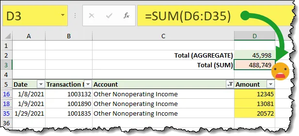
The AGGREGATE function allows you to sum (along with other functions like AVERAGE, COUNT, MAX, MIN, etc.) a range of cells while ignoring any cells that may contain errors as well as ignoring hidden values due to hiding rows and/or columns.
Take the following as an example:
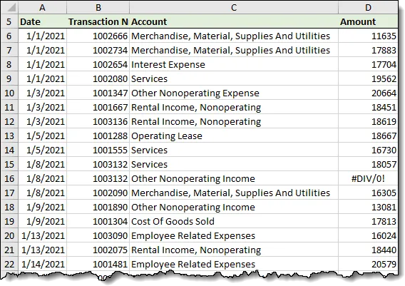
If we sum the entire range of “Amount” values, we will receive an error due to the one cell containing a “#DIV/0” error acting as a poison pill for the entire range.
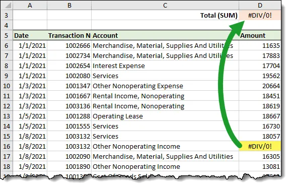
The AGGREGATE function will handle this without issue.
The AGGREGATE function is the Swiss Army Knife of functions.
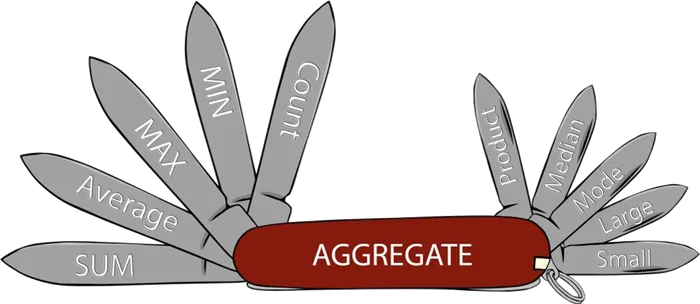
AGGREGATE is 19 separate functions packaged into a single function with additional features thrown in for good measure.
When you write a formula using the AGGREGATE function, you use a code number to indicate which of the 19 functions you wish to use.
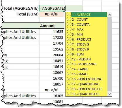
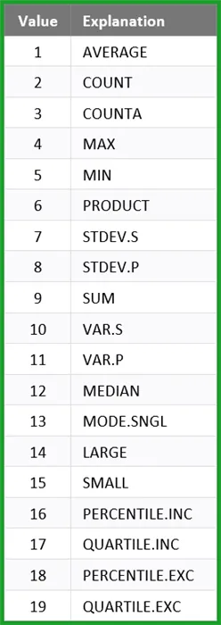
Selecting one of the numbers listed is no different than using the selected function on its own.
The benefit of using AGGREGATE comes with the next set of options.

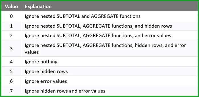
Selecting the appropriate option value will alter the way AGGREGATE behaves when encountering errors, hidden rows, or even other AGGREGATE functions.
This is a great way to create subtotals and grand totals whereby the grand totals ignore the subtotals, avoiding the issue of double counting.
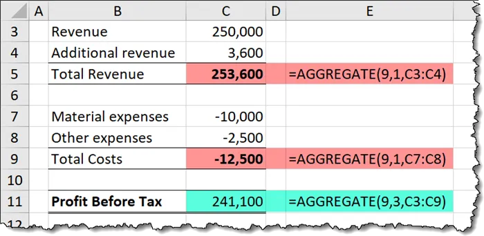
These options are also useful for when you are filtering tables and you don’t want the hidden rows to be included in the aggregations. The SUM function (along with other functions like AVERAGE, COUNT, MAX, MIN, etc.) would continue to include the values in the filtered/hidden rows.
If we were to filter the data and some of the remaining rows contained errors, the function would not only ignore all the “filtered out” rows, but also ignore the errors that remained.
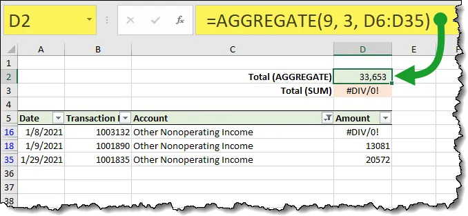
Even if the errors were not present, a traditional SUM function would continue to add all the selected rows regardless of the filtered state of the range.
Featured Course
Fundamentals of Financial Analysis

ROUND
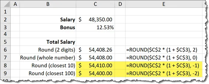
The ROUND function allows you to round your results to a set number of decimal places.
When we perform calculations, often the result is displayed to a level of precision beyond our needs.

To ensure that a result is only ever displayed to a set level of decimal precision, we can enclose the calculation in a ROUND function and define the number of decimal places, such as 2 decimal places…

…or rounded to a whole number.

A lesser-known ability of the ROUND function is that you can round UP in a “left of the decimal” fashion. This is useful when you are representing very large numbers, but you only need precision to a certain level.
Featured Course
Excel Essentials for the Real World

EMONTH
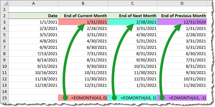
The EOMONTH (End of Month) function accepts a date or a reference to a cell holding a date and produces a new date that is the last day of the month for a set number of months forward or backward in time.
For example: If we supply the date “1/15/2021” and ask for the end of the month 3 months from that date, we will produce “4/30/2021” as a result. We move 3 months into the future then push to the end of the resultant month.
If we want the end of the current month, we inform EOMONTH to move 0 (zero) months forward.
If we want to move backward in time, we provide a negative value to the EOMONTH function.
BONUS FUNCTION
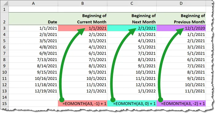
Unfortunately, Excel does not possess a BOMONTH (Beginning of Month) function, but with a bit of creativity, we can create one.
If you wanted to get the first date of the following month, you can write an EOMONTH function to calculate the end of the current month… then add a day.
EDATE
The EDATE function allows you to move a set number of months forward or backward in time based on a specified date.
Suppose we need to calculate warranty expirations based on the 14 months from the date of purchase.
The formula(s) would appear as follows:
=EDATE(A3, 14)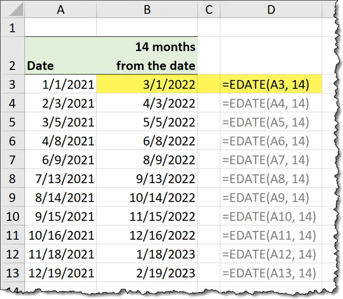
If you need to calculate N-number of months in the past, define the “Months” argument as a negative value.
=EDATE(A3, -14)If you wanted to be generous with your warranties and allow a grace period to the end of the 14th month, you could nest the EDATE function within in EOMONTH function.
=EOMONTH(EDATE(A3, 14), 0)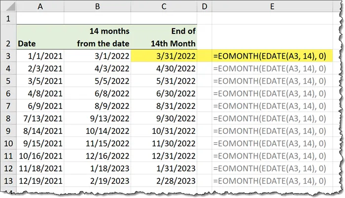
WORKDAY
The WORKDAY function is ideal for calculating a set number of days forward (or backward) in time but skip the weekends and possibly holidays. There are two versions of the WORKDAY function:
- WORKDAY – Older version that defines Saturday and Sunday as weekends.
- INTL – Updated version that allows for the definition of 1 or 2-day weekends and what day they occur.
As the WORKDAY.INTL is more feature-rich, we’ll demonstrate that version. We define the arguments as follows:
- Day to calculate from
- Number of days to count forward or backward
- The desired weekend combination
- The list of holidays (if needed)
If we have a date in cell A3 and we wish to count 21 days into the future, avoiding weekends (Saturday and Sunday) and any holidays that listed (range F3:F15), the formula would be written as:
=WORKDAY.INTL(A3, 21, 1, $F$3:$F$15)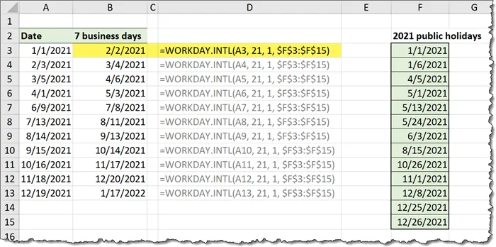
The codes for the weekends are as follows:
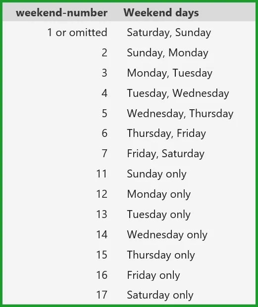
To learn more about the WORKDAY and NETWORKDAY functions, check out the link below.
XelPlus – WORKDAY & NETWORKDAY Functions explained
Featured Course
Master Excel Power Query – Beginner to Pro

3D Formulas
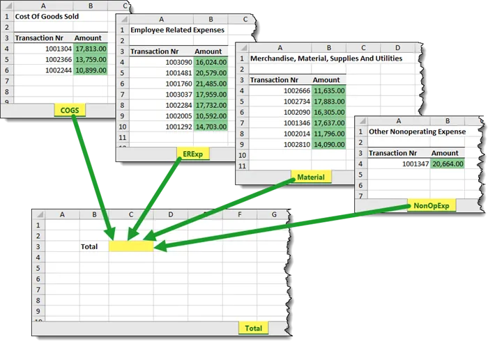
3D Functions aren’t functions but rather shortcuts to writing functions. Suppose you have several sheets of values that you need to sum together and place as a total on a separate sheet.The long way to write a formula like the following that references each sheet separately.
=SUM(COGS!B4:B15) + SUM(ERExp!B4:B15) + SUM(Material!B4:B15) + SUM(NonOpExp!B4:B15)Just like you can define a range of cells (ex: A1:A10) you can define a range of sheets (ex: COGS:NonOpExp).
We could rewrite the formula using a sheet range definition as follows:
=SUM(COGS:NonOpExp!B4:B15)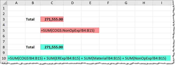
I great advantage to building a sheet range reference is, just like cells, if you were to insert something in between the starting and ending sheets, the data will be incorporated by the existing formula.
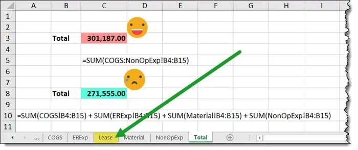
For more examples and detailed explanations of 3D formulas, check out the following link.
XelPlus – Excel 3D Formulas
SUMIFS / AVERAGEIFS / COUNTIFS
Think of the SUMIFS, AVERAGEIFS, and COUNTIFS functions as SUM, AVERAGE, and COUNT with built-in filters.
We can point to a range of cells and then define criteria by which to include specific items in the range.
For example:
- Sum amounts where the “Account” is equal to “Services”.
- Average “Profit” for discounted items.
- Count “Sales” that are more than “10,000”.
You can even define multiple filter criteria, such as sum the “Sales” over “100” for “Domestic” orders.
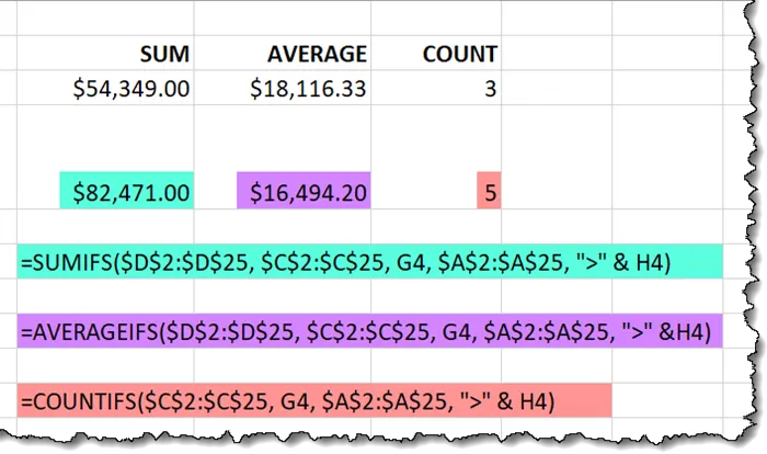
In the below example, we want to total all “Amount” cells (D2:D25) that are associated with the “Services” account (C2:C25). The formula would appear as follows:
=SUMIFS(D2:D25, C2:C25, "Services")If the “Services” account were listed in a cell (ex: G3), the formula could be written more dynamically like so.
=SUMIFS(D2:D25, C2:C25, G3)
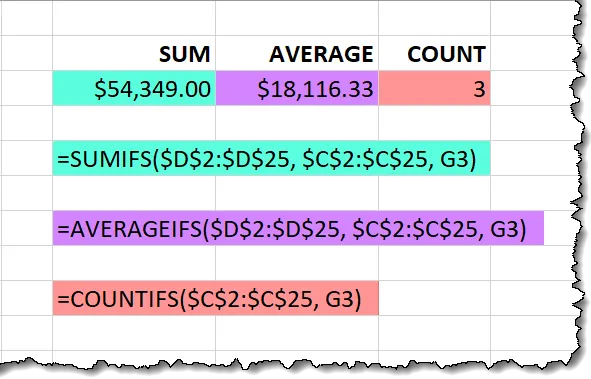
If we want to add another condition to the filter where the “Account” (C2:C25) must be “Employee Related Expenses” (G4) and the “Date” (A2:A25) must be after “1/15/2021” (H4).
We can write the formulas as follows:

To see more examples with detailed explanations of these functions, take a look behind these links:
XelPlus – How to SUM Different Columns based on Header?
XelPlus – Do you know the difference between the SUMIF and SUMIFS function?
IF
The IF function allows you to ask a question then act in one of two ways based on the answer.
The question you ask must be answerable as “True” or “False” and nothing else.
The formula looks like so: ask a question, then perform action “A” if true or perform action “B” if it’s false.
In the below example, we want to audit any “Amount” over “20,000”. We could say, “If the value in cell D2 is greater than 20000 then display the word “Check”. Otherwise, display nothing.”
=IF(D2 > 20000, "Check", "")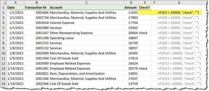
We can see that any amount more than 20,000 displays the “Check” message, while other cells display nothing.
NOTE: The use of the 2 double quotes is Excel’s way of saying “display nothing” (empty text).
PRO TIP: It’s best to place the 20,000 value in a separate cell and reference the cell as opposed to hard-coding the 20,000 into the IF formula. This way, you can more easily see what the “Amount” threshold is and if you need to change the threshold, you can change the single-cell value and update all the IF formulas in a single update.
=IF(D2 > H1, "Check", "")You can check for multiple conditions by either nesting an IF within another IF (you can do this up to 64 times) or you can use an IFS function that allows up to 127 logical declarations, although this is not recommended. Once you get past needing 10 or more decisions, there are usually alternate strategies that will perform better with less logical construction.
To see an ingenious use of wildcards for performing partial text matches with IF, check out the link below.
XelPlus – Excel IF Function with PARTIAL Text Match (IF with Wildcards)
Featured Course
Master NEW Excel Functions in Office 365 & Office 2021

VLOOKUP
The VLOOKUP allows you to take a value in one list, locate that value in another list, then return an associated piece of information.
It would be like ordering lunch where you locate an item in the menu, then return the price to see if you can afford the item.
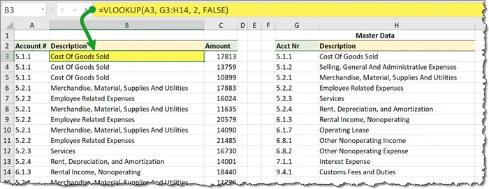
In our example below, we have a list of “Account #” (column A) and need the associated “Description” in column B.
A separate table has the “Account #” (column G) and “Descriptions” in column H.
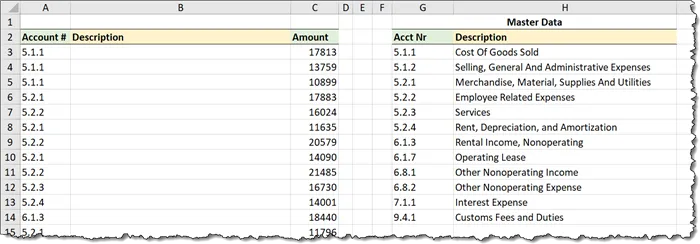
We can write a VLOOKUP formula that says, “Take the “Account #” in cell A3 and locate it in “Master Data” table (columns G:H). When found, move over to the 2nd column in the “Master Data” table and return the item on the same row.”
=VLOOKUP(A3, G3:H14, 2, False)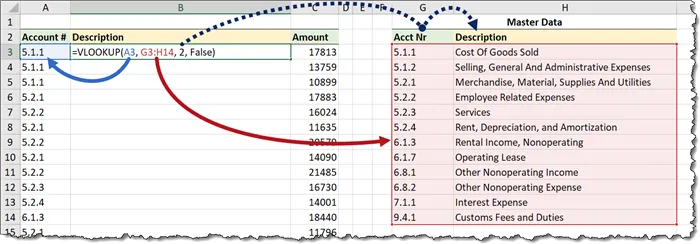
The “False” argument at the end tells VLOOKUP to locate the “Account #” exactly, otherwise, return an error message. If you are looking for items that are “close” to the object being searched for, you can write “True” here or leave it empty. This equates to what is known as an “Approximate Match” compared to an “Exact match”.
NOTE: When constructing the table to be searched (G3:H14) ensure that the leftmost (i.e., “first” column) contains the data to be searched. This is a requirement of the VLOOKUP function. The column of associated data being returned does not need to be directly next to the “first” column, but it does need to be to the right of the “first” column.
To see more examples of VLOOKUP (and HLOOKUP) in action, click the following link for some great practical examples of the functions.
XelPlus – VLOOKUP & HLOOKUP for Dynamic Lookups
AMAZING NEWS!!!!
If you are running a Microsoft 365 (formerly known as Office 365) subscription version of Excel, you have access to a new lookup function called XLOOKUP.
XLOOKUP is much more flexible, feature-rich, and easier to use. Check out these videos to learn more about this amazing new function.
XelPlus – Learn more about XLOOKUP on XELPLUS.com
TRIM
The TRIM function will remove any extra spaces either before or after the cell text as well as remove and redundant spaces within the text.
For example, if we had the following in cell A1:
“ This is a test ! “We could write the following formula:
=TRIM(A1)… and get returned “This is a test!”
This is a function to use when you are using VLOOKUP because sometimes the data being searched for has “invisible” spaces at the end that cause havoc with VLOOKUPs ability to perform an accurate match.
If we used the previous VLOOKUP example, we could make the formula more robust by nesting a TRIM function in the first argument like so.
=VLOOKUP(TRIM(A3), G3:H14, 2, False)Examples of creative uses of the TRIM function can be seen in the following post.
XelPlus – Removing “Stubborn” Spaces in Excel Data
Announcement for Office 365 Users (Time saver for Accountants)
All the above-mentioned functions are available in ALL versions of Excel. If you are an Office 365 subscriber, you have access to an assortment of new functions.
Check out this video that showcases many of these new functions. They are bound to change your Excel life.
XelPlus – Excel 365 Functions for 2021
Leila Gharani
I'm a 6x Microsoft MVP with over 15 years of experience implementing and professionals on Management Information Systems of different sizes and nature.
My background is Masters in Economics, Economist, Consultant, Oracle HFM Accounting Systems Expert, SAP BW Project Manager. My passion is teaching, experimenting and sharing. I am also addicted to learning and enjoy taking online courses on a variety of topics.


