#1 – Power Query Editor Launcher
This one is very simple, and only saves a few clicks. But if you open the Power Query editor over and over again, saving a few clicks here and there over time ends up amounting to a faster workflow.
To open the Power Query Editor, press the ALT-F12 keys combination on the keyboard.

If you happen to have your cursor sitting in the output of a query, ALT-F12 will open the Power Query Editor and place you on the last step of the query that produced that output.
#2 – Power Query Quick Access Toolbar Customization
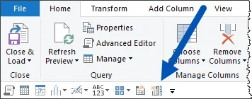
Power Query has a customizable Quick Access Toolbar (or QAT for short) just like regular Excel.

It’s not as feature-rich as the QAT in Excel, but it can be a great way to consolidate your most used Power Query actions into a single one-stop shop.
To add a feature to the Power Query QAT, right-click a feature on a ribbon and choose “Add to Quick Access Toolbar”.

Over time, you will have curated the perfect place to access your most saved features.

You can remove a feature from the QAT by right-clicking an icon and selecting “Remove from Quick Access Toolbar”.
You can also move the QAT below the ribbon to provide more room if you are inclined to add more buttons that the Toolbar would care to support. To do this, right-click any button on the QAT and select “Show Quick Access Toolbar Below the Ribbon”.

Featured Course
Automate With Power Query – Recipes to solve business data challenges

#3 – Avoid IntelliSense Errors by Not Typing the Dot
When writing formulas using Power Query functions, we are presented with the same formula writing assistant known as IntelliSense. This is the service that offers suggested function names as well as helpful insights into the needs of a function.
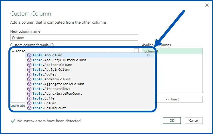
Power Query’s IntelliSense service is going through a bit of an awkward teenage phase where it thinks it knows what to do but often gets a bit confused.
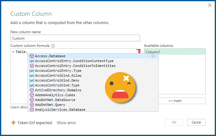
It’s not uncommon for the service to spin off into a wildly unrelated area of function name offerings after you type the dot that separates the function category from the function name.
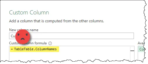
Another strange behavior is when you are typing a function (say the table function named “ColumnNames”), pressing Tab when selecting the offered function will unexpectedly double up the function category name.
The trick to keeping IntelliSense on the right track is to NOT TYPE THE DOT that falls between the category and name. It sounds odd, but it actually works.
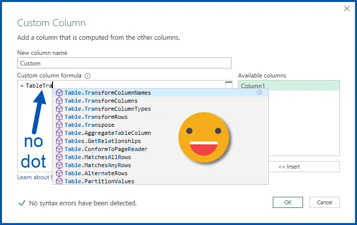
Once you see the function you’re interested in, arrow down to its position and hit the TAB key to complete the statement.
BONUS TIP – Accessing Power Query Function Help
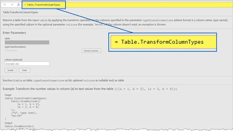
If you ever need help with understanding the layout or requirements of a specific function, write a formula in the Formula Bar that starts with an equals sign, then has the function name WITHOUT parentheses.
This will present the same content found on the Microsoft Power Query M Function Library website.
Featured Course
Master Excel Power Query – Beginner to Pro

#4 – Zoom in and Out Using Keyboard Shortcuts
One of the main frustrations Power Query users with large monitors have is that the fonts and information may be too small to easily read.

An easy way to zoom into the content is by pressing the CTRL-Shift-plus and CTRL-Shift-minus keys.

Each press of these key sequences will either increase or decrease the zoom factor of the Power Query Editor data interface.
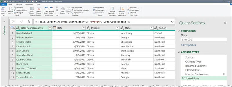
This is especially helpful when working with the Advanced Editor and viewing the query’s M code in its entirety.
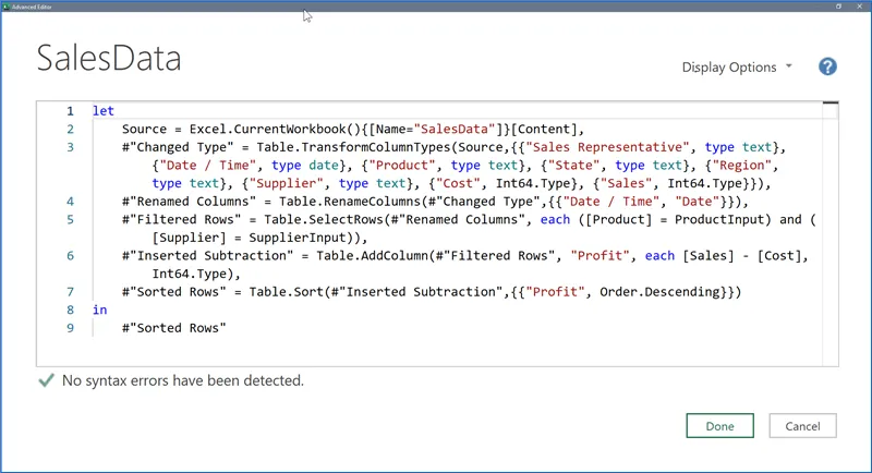
BONUS TIP: When operating in regular Excel, you can use the CTRL key in conjunction with spinning the mouse wheel to zoom in and out of a spreadsheet. Try it out; it’s crazy fun.
#5 – Sort Columns Alphabetically Using Power Query
When working with a table that has many columns, and you need to sort a table’s columns in alphabetical order, perform this set of quick steps to achieve a sorted list of column names.
- Start with an unsorted data set.

- Bring it into Power Query.
- Select Home (tab) → Manage Columns (group) → Choose Columns.

- Sort the displayed list by Name instead of Natural Order.
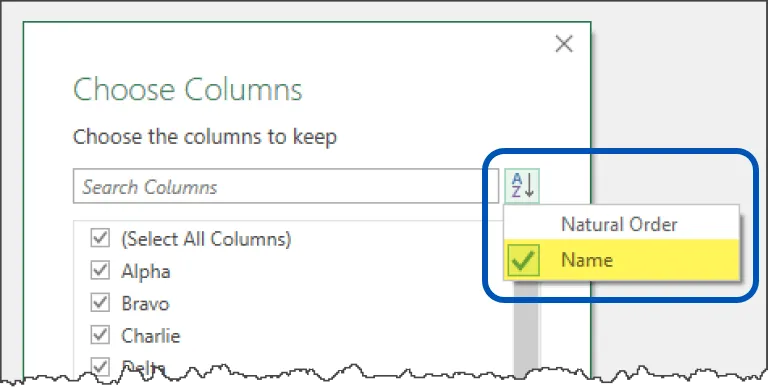
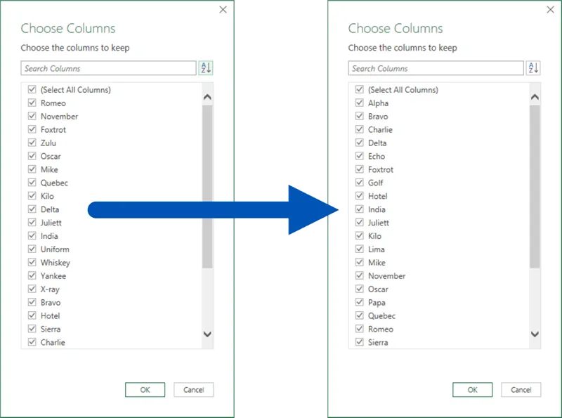
- Click OK and enjoy your newly sorted table.

#6 – Get All Excel Sheets by Selecting the Folder
When working with the “From Excel Workbook” data connector, an initial list of all sheets, tables, and ranges is presented in a Navigator window. This allows the user to select which worksheet, table, or range of data to be brought into Power Query for transformations.
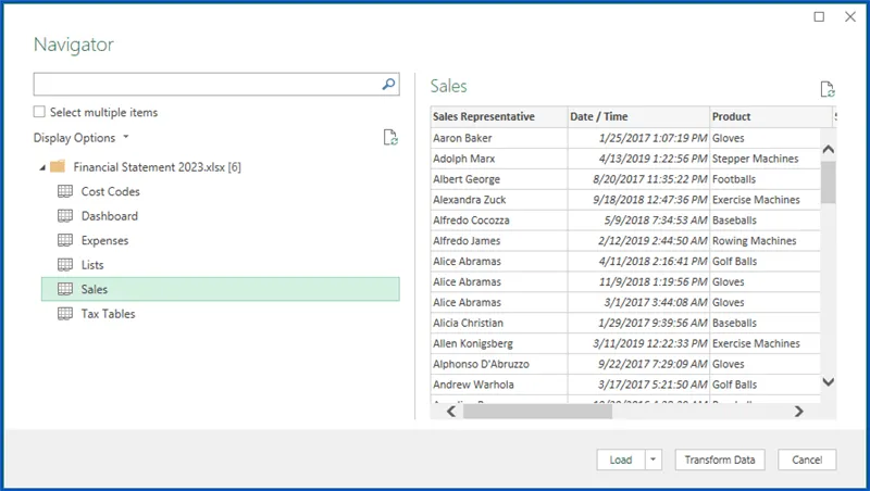
But what if multiple items from this list need to be brought into Power Query? Creating a separate query for each item would prove tedious and time-consuming.
Checking the box labeled “Select multiple items” will allow checkboxes to be used to select as many or as few items as needed.
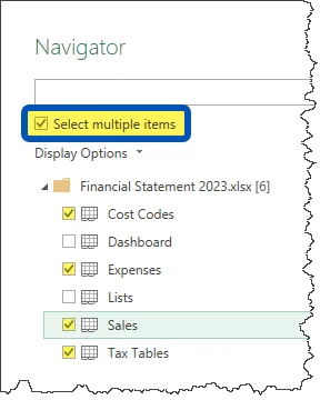
But what about the situation where new sheets are being periodically added and the user always needs every sheet in the file?
The trick is to select the folder icon next to the file’s name.
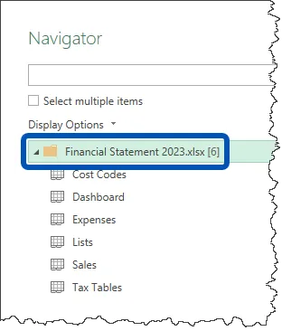
This will bring in a table of meta-data information about the objects on the list.

From here, creative filtering and selecting can reduce the list down to the items needed, then let the transformations FLY!
You can apply the same logic – use the folder – when connecting to other file types, such as PDF.
#7 – Change and Monitor Table Names from the QAT
When working with proper Excel Data Tables, it’s common to give the table a more memorable name. This makes writing formulas and referencing columns more intuitive.
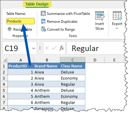
However, when you need to remember what you named a table, you must perform the following steps:
- Click on the table
- Select the Table Design ribbon
- Examine the Table Name field in the Properties group.
To ALWAYS see the table’s name, add the Change Table Name feature to the QAT.
- Right-click any button on the QAT and select “Customize the Quick Access Toolbar”.

- In the Customize Toolbar section, set the “Choose Commands From” dropdown to “Table Tools | Table Design Tab”. Select “Change Table Name” from the list and press the Add button (middle) to place the option on the right-side table. Click OK when done.
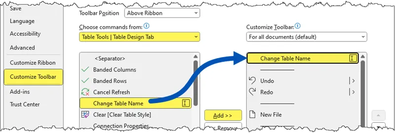
Alternatively, you can right-click “Table Name” in the Table Design Ribbon and click “Add to Quick Access Toolbar” to add the feature to the QAT.
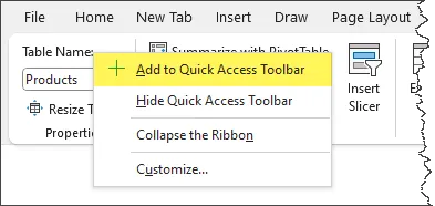
Either of these methods will add the below-displayed information onto the QAT.
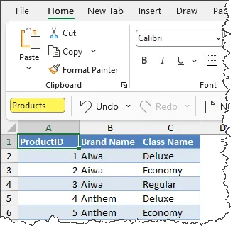
It’s now much easier to keep track of the selected table’s name as well as update the name when needed.
Featured Course
Fast Track to Power BI

#8 – Copy and Paste Queries Between Excel Files
One of Power Query’s great strengths is to reduce the amount of repetitive work. Writing a query and then repeating all the transformation steps with a single click of the “Refresh” button.
But what if you have a lengthy query with dozens of steps, and you need to build a query in a different file that serves the same or similar purpose?
Power Query allows users to copy and paste queries from one file to another. It’s easy.
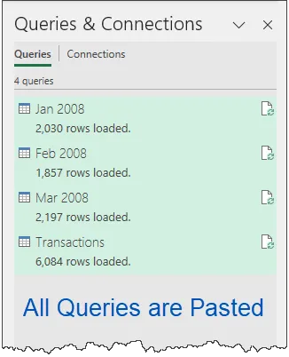
Open a file with the source query and display the Queries & Connections panel (located on the Data ribbon).

From the Queries & Connections panel, right-click the needed query and select Copy.
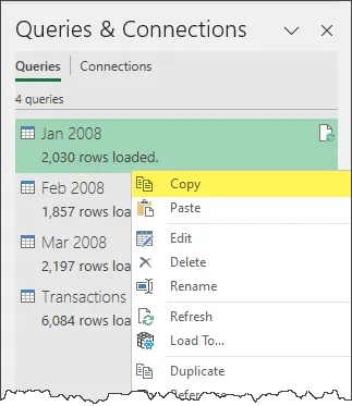
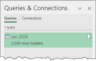
Navigate to the destination file, activate the Queries & Connections panel, then right-click in an empty part of the panel to select Paste.

Now bask in the glory that is your new, complete query.
BONUS COPY TIP
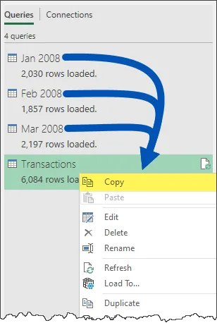
If you copy a query that is dependent on the output of other queries (known as “feeder queries”), the selected query along with all “feeder queries” will be pasted to the destination file.

#9 – Add Excel Slicers to Tables
Power Query’s output often takes the form of proper Excel Tables. Because of this, Slicers can be used to easily filter the table.
If you haven’t heard of Slicers, think of them as super-fast filters. Instead of wandering through lengthy lists of checkbox items, Slicers present easy-to-read and easy-to-select buttons.
Take the below Power Query output table for example.
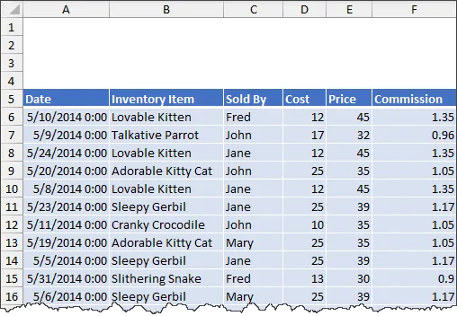
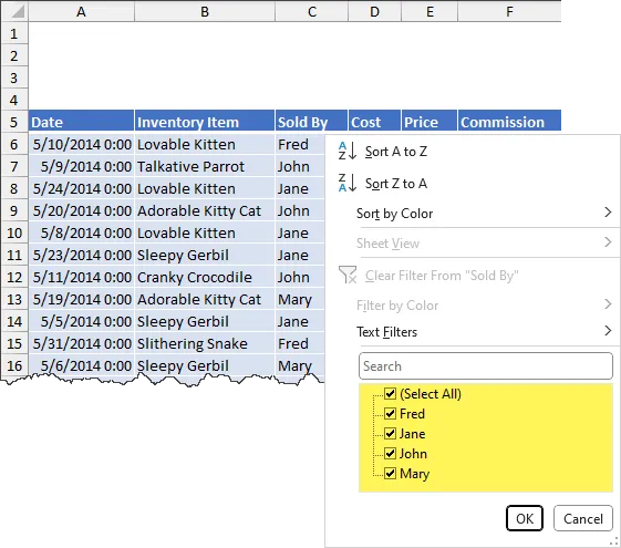
If we wish to filter by the [Sold By] column, we could use the old-school checkbox filter controls.
Or we could add a Slicer to perform the filtering.
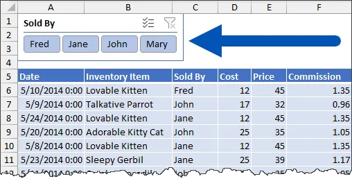
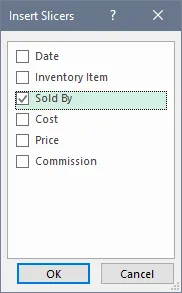
To add a Slicer to a proper Excel Data Table, click the table, then select Table Design (tab) – Tools (group) – Insert Slicer.

Select the field (or fields) you wish to use as Slicer controls.
The initial Slicer offering is rarely in the size, location, or color that you wish it to be.
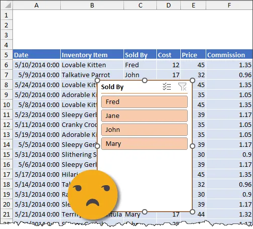
Use the resize handles to shape the Slicer to the desired height and width, then move the slicer to the desired location.
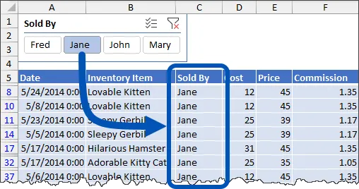
You can use the Slicer ribbon to apply various other customizations, like color, name, heading customization, number of columns, etc.

Clicking one of the buttons will instantly filter the table.
#10 – Adjust Power Query Refresh Settings
Suppose you have a Power Query result that needs to be updated each time the Excel file is opened. Or how about every twenty minutes while the file is open?
We can’t expect the user to click the Refresh button every twenty minutes.
This refresh process can be automated by opening the Queries & Connections panel (located on the Data ribbon), then right-clicking a query and selecting Properties.
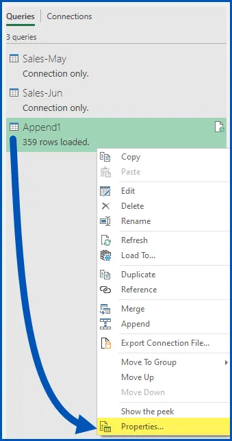
In the Query Properties dialog box, select the best refresh option that meets your needs.
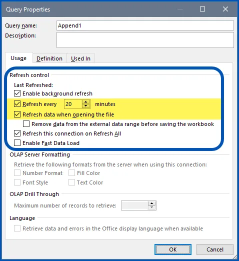
Each query can be controlled differently, giving you maximum flexibility when updating workbooks with multiple queries.
Closing Thoughts
The above tips are but a tiny fraction of ways you can optimize your Power Query workflow while at the same time dazzling your supervisors and coworkers.
For more information on how you can become the best Power Query user imaginable, check out my courses listed below for both beginners and advanced users.
Leila Gharani
I'm a 6x Microsoft MVP with over 15 years of experience implementing and professionals on Management Information Systems of different sizes and nature.
My background is Masters in Economics, Economist, Consultant, Oracle HFM Accounting Systems Expert, SAP BW Project Manager. My passion is teaching, experimenting and sharing. I am also addicted to learning and enjoy taking online courses on a variety of topics.


