Digging Deeper Into the Data
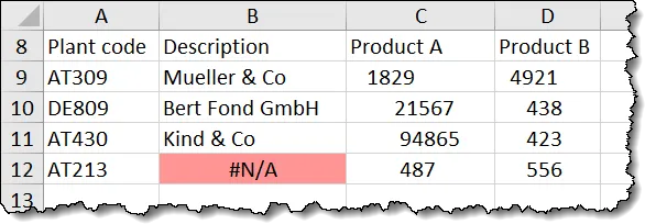
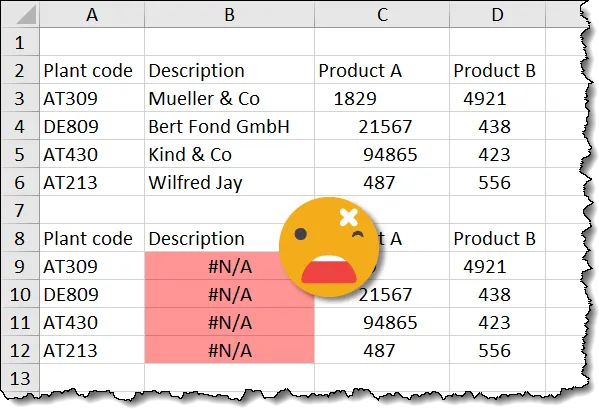
Why does this newly copied and pasted dataset fail?
The formula appears to be correct.
=VLOOKUP(TRIM(A9), $G$3:$H$7, 2, FALSE)If we highlight the TRIM function portions of the formula and press F9, we can clearly see a space at the end of the search value.

Why did the TRIM function fail to remove this trailing space?
Although the TRIM function removes spaces, there are a variety of types of spaces, and TRIM can’t deal with all types.
The TRIM function removes spaces which are generated using the ASCII code of 32.
SIDEBAR: The American Standard Code for Information Interchange (ASCII) code table is a character encoding standard for electronic communication. ASCII codes represent text in computers, telecommunications equipment, and other devices as numbers. For example, the capital letter “A” is represented in the ASCII table as the number 65, “B” as 66, and “C” as 67, etc. The “space” character is represented as the number 32.
There is, however, another type of “space” character known as a non-breaking space that is represented by the ASCII code number 160.
An Interesting Test
If you want to see the code number that hides behind a character, type a character in a cell (like the capital letter “A” in cell A1), then select another cell and write a formula like the following
=CODE(A1)The CODE function displays the ASCII code for the first character in a string detected in the target cell.
If we were to highlight and copy the trailing space from the value in cell A9 and paste it into our test cell, the CODE function sees it as ASCII code 160.
This non-breaking space is common amongst data that is copied from sources such as email readers, word processors, and web browsers.
Seeing Things from the Opposite Side
Another Excel text function is the CHAR function. This function takes an ASCII code number and represents it as its “human-friendly” version.
=CHAR(32) or =CHAR(160)The above formulas will generate a traditional “space” and a non-breaking “space”.
To our eyes, these both look the same, but Excel sees them as completely different characters, no different than seeing “A” and “B” as different characters.
The TRIM function can remove ASCII 32 characters but not ASCII 160 characters.
Improving the TRIM Function
Until Microsoft releases a version of the TRIM function that can deal with all types of spaces (TRIMALL sounds like a catchy name), we will have to take matters into our own hands and develop a more robust formula that can work with both types of characters.
If we ask ourselves, “How can we get TRIM to see the character 160s as character 32?” This sounds like the job of a Find/Replace action.
Excel has a function that can replace text with different text: the SUBSTITUTE function.
The SUBSTITUTE Function
The SUBSTITUTE function will search a cell for a defined text string and replace it with another text string. An example would be as follows:
=SUBSTITUTE(A1, "Microsoft", "XelPlus")There is an optional 4th argument that allows you to specify exactly which occurrence in the text to replace, such as “only the 3rd occurrence”.
=SUBSTITUTE(A1, "Microsoft", "XelPlus", 3)If you omit this 4th argument, all occurrences are replaced.
Updating Our Formula
Remember our original lookup function?
=VLOOKUP(TRIM(A9), $G$3:$H$7, 2, FALSE)Let’s begin by taking out the TRIM function and putting in its place a SUBSTITUTE function.
=VLOOKUP(SUBSTITUTE(A9, CHAR(160),), $G$3:$H$7, 2, FALSE)“But wait! You forgot to replace the non-breaking space with a normal space.”
It’s easy to think that would be the required step, but why replace a non-breaking space with something we ultimately want to throw away?
=VLOOKUP(SUBSTITUTE(A9, CHAR(160), CHAR(32)), $G$3:$H$7, 2, FALSE)We got a bit crafty here and replaced the non-breaking space with nothing, which is a legal move and more efficient because it achieves what would have been a 2-step process in a single step.
If we fill the updated function down the list, we see that it works in most cases, but fails in a few.

This is because the SUBSTITUTE function is not searching for regular spaces to change to nothing.

Our solution is to give the SUBSTITUTE function a “first pass” at extracting non-breaking spaces, but afterward, give the TRIM function a “second pass” to catch any normal spaces.
=VLOOKUP(TRIM(SUBSTITUTE(A9, CHAR(160),)), $G$3:$H$7, 2, FALSE)Aggregating Values with Spaces
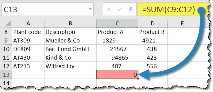
Suppose we wanted to SUM all the values for “Product A” in our table.

The SUM function returns 0 (zero) because it sees all the data as text.
The below image uses a series of ISTEXT functions to test the “Product A” cells to see if the data is perceived as text by Excel. As you can see, Excel returns TRUE responses for all the tests.

Another Excel text function called VALUE can read a number stored as text as a ‘normal’ number.
=VALUE(C9)Although the VALUE function ignores “space” characters, it fails to ignore non-breaking spaces.
If we nested the VALUE function within a TRIM function, it wouldn’t solve our problem.
=TRIM(VALUE(C9))We need to use the SUBSTITUTE function.
=SUBSTITUTE(C9, CHAR(160),)But the result is still not a usable number because the original text is still perceived as text. We need to convert the text to a real number using the VALUE function.
=VALUE(SUBSTITUTE(C9, CHAR(160),))When to Use
Whenever you encounter data where…
- your numbers are not being perceived as numbers,
- you use the TRIM function and it fails,
- you use the VALUE function and it fails,
…use the SUBSTITUTE function to search for character code number 160 and replace it with “nothing”.
Get Fancy with a Single Step Solution
Instead of creating a pre-processed version of the data to then aggregate, we can perform the conversion and aggregation in a single step.
=SUM(VALUE(SUBSTITUTE(C9:C12, CHAR(160),)))If you are working with the new Dynamic Array version of Excel, this formula works perfectly.
If you are working with an older (pre-Office 365) version of Excel, you will need to write the formula the same way as before,
=SUM(VALUE(SUBSTITUTE(C9:C12, CHAR(160),)))..but you will need to commit the formula using the CTRL-Shift-Enter key combination instead of a normal Enter key.
This creates the formula as an array formula to enable the SUBSTITUTE function the ability to process multiple cells worth of data.
Practice Workbook
Feel free to Download the Workbook HERE.

Leila Gharani
I'm a 6x Microsoft MVP with over 15 years of experience implementing and professionals on Management Information Systems of different sizes and nature.
My background is Masters in Economics, Economist, Consultant, Oracle HFM Accounting Systems Expert, SAP BW Project Manager. My passion is teaching, experimenting and sharing. I am also addicted to learning and enjoy taking online courses on a variety of topics.


