Behold… Pete’s creation!!!!!!!!!!
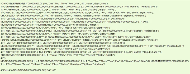
DON’T RUN AWAY JUST YET!
Don’t worry if this looks a bit intimidating; you don’t need to understand this to use it. We only need to know how to integrate it into our spreadsheets.
SCROLL DOWN TO DOWNLOAD THE WORKBOOK & CHECK OUT THE POWER QUERY SOLUTION TO THIS (sent to us by our wonderful community)
Let’s look at some examples


This formula is quite complex, having to account for such instances of where it sees values such as “Eleven” (as opposed to “One and One”), “Twenty”, “Thirty”, and weather to say things like “Hundred” versus “Hundred and” something.
The combination of numbers to words can be quite daunting.
Changing the Currency and Decimal Usage
Suppose you need to update this formula to work with US dollars and you don’t require the decimal places.
If you look at the very end of the formula, you will see the portion that is responsible for the decimal places.
&RIGHT(TEXT(B3,"000000000.00"),2)&"/100"
If you do not require decimal places to be displayed, erase this portion of the formula.
For the currency type, change the portion labeled “Euro” to “USD” or “CAD” or whatever currency designation you wish.

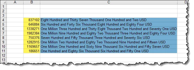
Let’s see how that appears after our little formula tweak.

How to apply the formula to many cells
Suppose you have a spreadsheet and you wish to enter a number in cell B4 and have the formula answer appear in the cell directly to the right in cell C4.
We need to make sure that none of the cell references change when copying the formula to a new location.
- Place your cursor on the cell holding the original formula and press F2 to enable edit mode (or click in the Formula Bar).
- Select the entire formula by pressing CTRL-A (or manually highlighting the formula. CTRL-A is faster and more accurate.)
- Press CTRL-C to copy the formula.
- Press the ESC (Escape) key to back out of edit mode.
- Switch to the location and cell you wish to use this formula and press F2 to enable edit mode.
- Press CTRL-V to paste the formula into the new cell.
We’re not quite there yet because all the cell references are pointing to cell B3. If your data entry cell is in fact cell B3, you are ready to go. If not, we need to update the cell references to point to the proper data entry location.
Because our original formula was looking at cell B3 for the number and we wish to enter our number in cell B4, we will now perform the following steps to adjust our cell references:
- Place your cursor on the cell holding the pasted formula and press F2 to enable edit mode (or click in the Formula Bar).
- Remove the equals sign (=) from the beginning of the formula.
- Press ENTER. We now have just a massive amount of text in the cell.
- Press CTRL-H to open the Find/Replace dialog box.
- In the “Find what:” field, enter “B3” (no double-quotes).
- In the “Replace with:” field, enter “B4” (no double-quotes).
- Press the “Replace All” button.
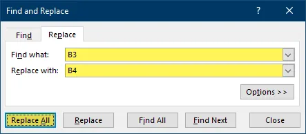
Restore the equals sign to the beginning of the formula from where we removed it earlier in step 2.
Running it through some tests
To test the formula quickly and over multiple iterations, select cell B4 and enter the following formula.
=RANDBETWEEN(1,2000000)This formula will generate a random number between 1 and 2-million each time the sheet recalculates.

You can force a recalculation by pressing the F9 key on the keyboard or pressing Formulas (tab) -> Calculation (group) -> Calculate Now.

To see several examples simultaneously, select cells B4 and C4 and pull the Fill Series handle down several rows. This will generate several random numbers and their text counterparts.
Bonus Modification
If you decide to not display the fractional side of the number, the above modification simply removes the fractional values without any rounding operation.
If you would like to round the input to the nearest whole number, implement the following steps:
- Place your cursor on the cell holding the pasted formula and press F2 to enable edit mode (or click in the Formula Bar).
- Remove the equals sign (=) from the beginning of the formula.
- Press ENTER. We now have just a massive amount of text in the cell.
- Press CTRL-H to open the Find/Replace dialog box.
- In the “Find what:” field, enter “B3” (no double-quotes).
- In the “Replace with:” field, enter “ROUND(B3,0)” (no double-quotes).
- Press the “Replace All” button.
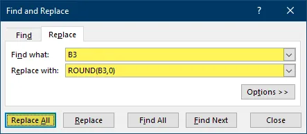
Restore the equals sign to the beginning of the formula from where we removed it earlier in step 2.
Don’t forget to change the B3 reference to whichever cell you are performing the data entry.
Are you curious as to how all this works?
This formula relies on the use of four key functions:
- LEFT
- MID
- TEXT
- CHOOSE
It’s not necessary to dissect every component of the formula, we only need to decipher the first bit highlighted below.

CHOOSE(LEFT(TEXT(B3),"000000000.00"))+1,,"One","Two","Three",
"Four","Five","Six","Seven","Eight","Nine")
&IF(--LEFT(TEXT(B3),"000000000.00"))=0,,IF(AND(--MID(TEXT(B3),"000000000.00"),
2,1)=0,--MID(TEXT(B3),"000000000.00"),3,1)=0)," Hundred"," Hundred and "))
Once we have this portion figured out we’ll be able to figure out the remainder of the formula since it is very much a repeated operation.
The LEFT Function
The purpose of the LEFT function is to extract a specific number of characters from the text starting from the left side. The structure of the LEFT function is as follows.
=LEFT(text, [num_chars])The parameter “text” refers to the cell holding the input, while “[num_chars]” indicates the number of characters to extract. Because the “[num_chars]” parameter is optional, skipping this parameter will result in a default extraction of 1 character.
The MID Function
The purpose of the MID function is to extract a specific number of characters from the text starting from a specific character position (counting from the left side). The structure of the MID function is as follows.
=MID(text, start_num, num_chars)The parameter “text” refers to the cell holding the input; the parameter “start_num” indicates the position to begin text extraction (counting from the left side), while “num_chars” indicates the number of characters to extract.
The TEXT Function
The purpose of the TEXT function is to represent a cell’s information with specific formatting. The structure of the TEXT function is as follows.
=TEXT(value, format_text)Normally, formatting is applied to a cell through traditional cell formatting controls.
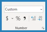
The TEXT function applies formatting (fancy word alert) formulaically. This way, we can change the formatting of information dynamically based on the need of the moment.
EXAMPLE: Suppose you have a calculation that needs to reflect U.S. Dollars or Euros depending on a country selection. The formula could look something like the following:
=IF(Country=”USA”, TEXT(Sale, ”$#,##0.00”), TEXT(Sale, “€#,##0.00”))If the user selects USA (cell A2) , they get the total sales represented by a “$” sign (cell C4) . If the user selects any other country, the total sales is represented by a “€” symbol.
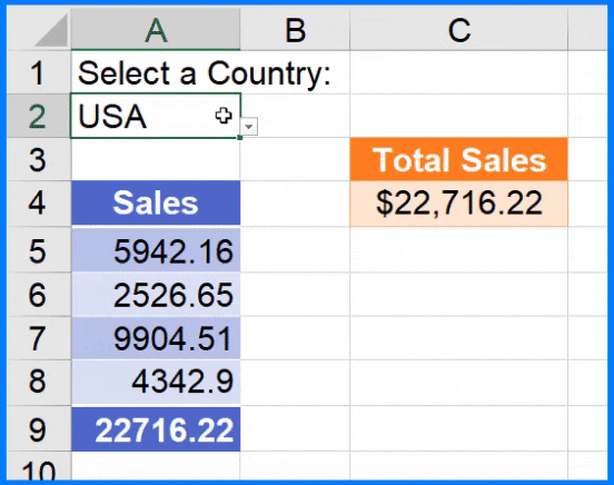
This function relies on a cell named “Country” (cell A2) where a user may select a country from a Data Validation dropdown list, and a cell named “Sale” (cell A9) that may hold something like a SUM function that adds all the sales together.
In our specific example, the function…
=TEXT(B3,”000000000.00”)…pads the input number with leading zeroes. By counting the leading zeroes, the formula will be able to determine if the number is in the hundreds, thousands, or millions.
If a user inputs a number, such as 123456.78, the TEXT function will interpret the number as 000123456.78. The three leading zeroes indicates a number in the thousands.
The CHOOSE Function
The CHOOSE function is used to simplify multiple nested IF functions that are examining the same data. CHOOSE is especially useful when working with indexes.
The purpose of the CHOOSE function is to select a value from a built-in list of values based on a supplied number.
=CHOOSE(index_num, value1, [value2], …)If we were to extract the first (left-most) number from the input number and give it to the following CHOOSE function, what do you think we would get back from the CHOOSE function?
=CHOOSE(LEFT(B3), “One”, “Two”, “Three”, “Four”, “Five”, “Six”, “Seven”,
“Eight”, “Nine”)
We would see the word version of the extracted number. “2” would yield “Two”, “5” would yield “Five”, etc…
Putting it All Together
In the formula, we are combining all the functions into a single formula, each function performing their respective parts to accomplish the mission.
CHOOSE(LEFT(TEXT(B3,"000000000.00"))+1,,"One","Two","Three",
"Four","Five","Six","Seven","Eight","Nine")
&IF(--LEFT(TEXT(B3,"000000000.00"))=0,,IF(AND(--MID(TEXT(B3,"000000000.00"),
2,1)=0,--MID(TEXT(B3,"000000000.00"),3,1)=0)," Hundred"," Hundred and "))
First we use the TEXT function to turn the number into a “000000000.00” format.
TEXT(B3,"000000000.00")Then, we extract the left-most character form the number.
LEFT(TEXT(B3,"000000000.00"))This will allow us to determine if the returned number is a zero or any other value. This will indicate weather or not our number is in the “millions” range.
Next, we CHOOSE how to represent the extracted value.
CHOOSE(LEFT(TEXT(B3,"000000000.00"))+1,,"One","Two","Three",
"Four","Five","Six","Seven","Eight","Nine")
We then check to see if the value is a zero.
CHOOSE(LEFT(TEXT(B3,"000000000.00"))+1,,"One","Two","Three",
"Four","Five","Six","Seven","Eight","Nine")
&IF(--LEFT(TEXT(B3,"000000000.00"))=0,,
If the value is a zero, then we are not in the millions so we will display nothing.
If the next two digits are zero, then we will display “Hundred”; otherwise, we will display “Hundred and”.
CHOOSE(LEFT(TEXT(B3,"000000000.00"))+1,,"One","Two","Three","Four",
"Five","Six","Seven","Eight","Nine")
&IF(--LEFT(TEXT(B3,"000000000.00"))=0,,IF(AND(--MID(TEXT(B3,"000000000.00"),
2,1)=0,--MID(TEXT(B3,"000000000.00"),3,1)=0)," Hundred"," Hundred and "))
That’s It!
This formula doesn’t rely on any
- VBA
- CTRL-Shift-Enter Array Formulas, or
- Helper Cells
Thank you, Pete for sharing your formula with the Excel community. I’m certain many will find your solution both creative and highly useful.
Practice Workbook
Feel free to Download the Workbook HERE.

Many thanks to Jim M. for updating the formula for US syntax, Zafar for updating it for billions as well as text as decimal places!
Also many thanks to Abdul Rahman Mohammed for providing the Qatari Riyals (QAR), Indian Rupees (INR) & Bahraini Dinars (BHD) in both absolute and rounded figures.
The reworked versions are available in the downloadable Workbook.
Power Query Solution!
A Power Query solution of transforming numbers to works was sent to us by Kunle SOPEJU.
Check out his Power Query solution HERE.

Many thanks to Kunle SOPEJU for letting us get creative with Power Query!
Leila Gharani
I'm a 6x Microsoft MVP with over 15 years of experience implementing and professionals on Management Information Systems of different sizes and nature.
My background is Masters in Economics, Economist, Consultant, Oracle HFM Accounting Systems Expert, SAP BW Project Manager. My passion is teaching, experimenting and sharing. I am also addicted to learning and enjoy taking online courses on a variety of topics.


