A while ago, I made a video/post called “10 Functions for Engineers” (link below) wherein one of the solutions a formula incorporated the LOOKUP function as part of its solution.

This was used to locate the immediate parent node in a hierarchy of nodes.
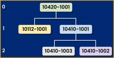
10 Excel Functions You NEED to KNOW as Engineers!
Several viewers commented that they wanted to better understand how the LOOKUP function operated in this scenario.
Let’s break it down to its core elements and then see if there is a more modern approach to solving the same problem.
Looking Up Data the “Old School” Way
The LOOKUP function is quite simple in its design. The syntax for LOOKUP is as follows:
LOOKUP(lookup_value, lookup_vector, [result_vector] )- lookup_value (required) – A value that LOOKUP searches for in the first vector. Lookup_value can be a number, text, a logical value, or a name or reference that refers to a value.
- lookup_vector (required) – A range that contains only one row or one column. The values in lookup_vector can be text, numbers, or logical values.
- result_vector (optional) – A range that contains only one row or column. The result_vector argument must be the same size as lookup_vector. It must be the same size.
To put it in plain English:
- What do you want to find?
- Where do you want to find it?
- What do you want to be returned?
Our example below shows a list of employee names and salaries.
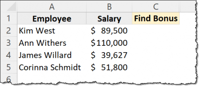
We wish to locate the employees’ salaries in a list of salary ranges to return a bonus percentage.
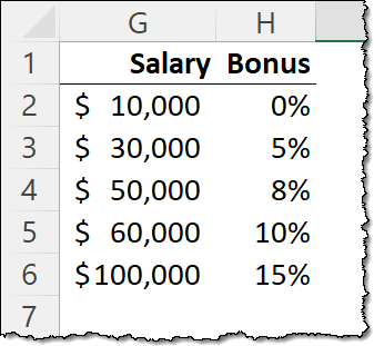
If an employee’s salary is not expressly defined in the Salary/Bonus list, we need to return the bonus where the salary is as close to the customer’s salary without going over (i.e., exceeding).
Example: If an employee has a salary of $49,000, the returned bonus would be 5%. Although $49,000 is closer to $50,000 than $30,000, the $50,000 cutoff exceeds $40,000. Thus, $30,000 is the closest salary on the list without going over $40,000.
Starting with Kim West’s entry (cell C2), we can write the following formula:
=LOOKUP( B2, $G$2:$G$6, $H$2:$H$6 )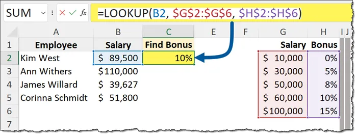
Note: The references to ranges G2:G6 and H2:H6 must be referred to absolutely so the references do not change when the formula is filled (i.e., repeated) to the adjacent rows below.
This appears to work perfectly.

Did you notice in the LOOKUP function there was no decision on whether the function should look for an exact match or an approximate match?
All uses of LOOKUP default to an approximate match. There is no option for limiting the logic to an exact match posture.
Important Point About the LOOKUP Function
One of the requirements for LOOKUP to operate properly is that the lookup_vector (in this case, $G$2:$G$6) must be sorted in ascending order.
If the list is stored in any other way, the LOOKUP function will almost certainly return either incorrect results or errors.

Strengths and Weaknesses
Suppose we need to locate the employee ID in the following table by using the employee’s name.
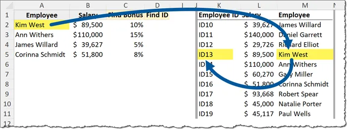
A more traditionally used lookup function like VLOOKUP would be unable to perform this operation without the help of other advanced functions like CHOOSE. This is because the results_vector lies to the left of the lookup_vector. This is a major league no-no with VLOOKUP.
On the other hand, because these vectors are defined explicitly by the LOOKUP function, a specific arrangement is not required.
Starting with Kim West’s entry (cell D2), we can write the following formula:
=LOOKUP( A2, $M$2:$M$11, $K$2:$K$11 )Regrettably, this did not produce the desired results.
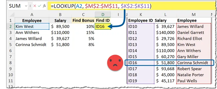
I’m sure you’ve already guessed that the reason for this inaccuracy is due to the sort order of the lookup data. The lookup table is sorted in ascending order by Employee ID, not by Employee (Name).
If we sort the lookup table in ascending order by Employee we are delivered the expected results.
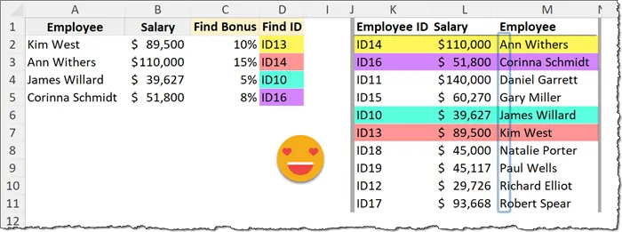
Remember, when using the LOOKUP function your lookup vector needs to be in ascending order.
Discovering Parent Nodes in a Hierarchical List
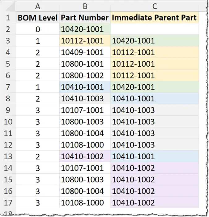
Working with a list of part numbers, we need to discover the part number that would serve as the parent part number for all its child part numbers.
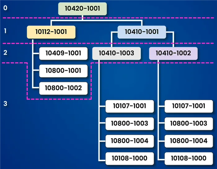
Below is a list of the part numbers and their associated BOM (Bill of Materials) Level.
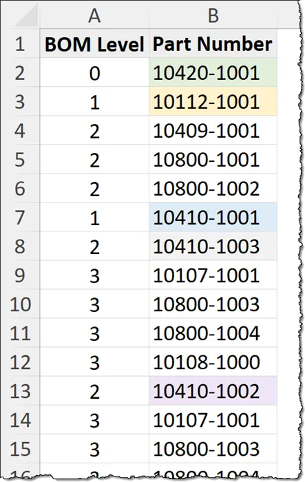
This is a bit of a tricky operation because we don’t want to discover each part number’s BOM Level value, we already know that rather the BOM Level number of its parent. Once we locate the parent’s BOM Level, we can discover the associated part number.
For example, if we are looking at a part number with a BOM Level of 3, we need to discover the part number at BOM Level 2 associated with that child.
As the part number at BOM Level 0 has no parent, we’ll skip that one for now.
Starting in cell C2, we write the following formula:
=LOOKUP( A3 – 1, $A$2:A3, $B$2:B3 )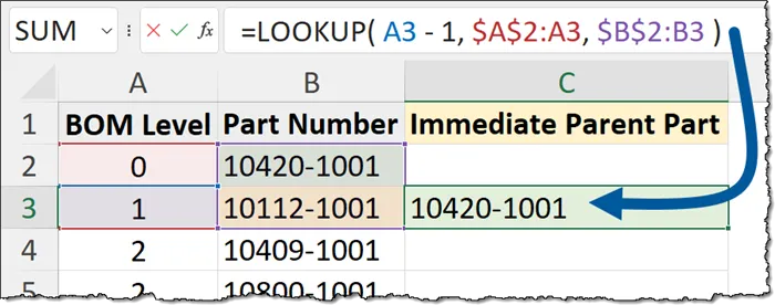
We have a couple of interesting and somewhat unconventional tactics happening in this formula.
- The lookup_value is having 1 subtracted from it. This allows us to search for the parent BOM Level value rather than the current BOM Level value as each parent is 1 less than their child.
- The range references for both the lookup_vector and the results_vector have the first portion fixed as an absolute reference (with the dollar signs) while the second portion is left as a relative reference (without the dollar signs).
The idea here is that when the formula is filled down to adjacent rows, the two vectors will expand to examine additional rows of content. This limits the search range to only values up to and including the current position in the list.
It’s the second tactic that is the most interesting, and possibly the most puzzling.
If we examined the entire range of data for both the lookup_vector and results_vector, the results would appear as follows.
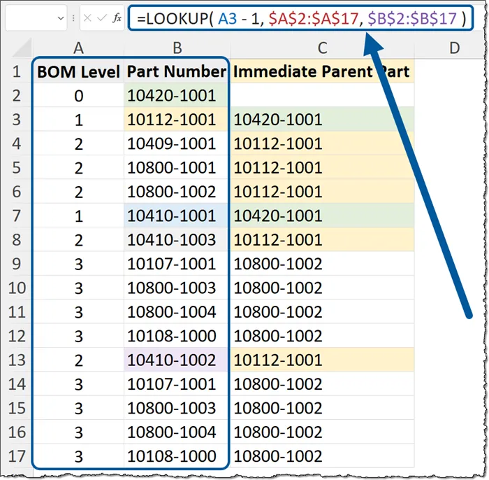
Each BOM Level 3 item is discovering “10800-1002” as its parent. This is because the LOOKUP stops when it encounters the first BOM Level 2 entry.
Granted, the first BOM Level 2 entry is in cell A4; we have a series of “2” values in cells A4 through A6. The LOOKUP function rests on the last entry on the duplicated series (cell A6). Thus, the part number in cell B6 (“10800-1002”) is returned for all BOM Level 3 entries.
The references used earlier where the first portion is set as absolute, and the second portion set as relative…
$A$2:A3 and $B$2:B3
… helps somewhat in combating this issue, but not much.
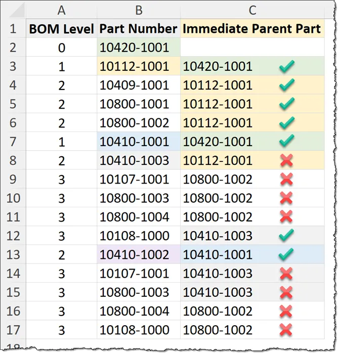
These incorrect results are due to 2 factors:
- Our BOM Level values are not sorted in ascending order.
- The direction that LOOKUP is performing the search.
LOOKUP is searching from the TOP DOWN. We need LOOKUP to search from the BOTTOM UP.
“But wait!”, you say. “Won’t that just cause the opposite problem?”
No, because the expanding range will always limit our search to only the current row and those rows previously examined.
We can’t sort the list by BOM Level, and the LOOKUP function is a bit lacking in configurable options, like searching from the bottom up. We need to get creative with our formula.
To help solve this problem, we will create our custom lookup vector that consists of “True/False”, then ultimately “1s/Errors”.
First, (ignoring the lookup_value for the moment) we modify the lookup_vector argument to compare each entry in the range to the BOM Level minus 1.

For the formula in cell C3, this would resolve each test as shown below; true and false.

PRO TIP: To see the results of each test, highlight the desired argument and press F9. Make certain you press Undo (CTRL-Z) to return the formula to its original state before leaving edit mode.
We need to turn these “true/false” results into “1s/Errors”. This is easily done by dividing each of the results into 1.

Our new test results are below.

This way of testing will only yield 1s and errors.
Looking at the last entry in the table (cell C17), the formula appears like so…

…and resolves each test in the following way.

Here’s Where the Magic Takes Place
Since an array of tests will only result in 1s and errors, we need only search for any value greater than 1, like 2.

LOOKUP will search the entire range for the number 2, never find it, then settle on the last number it saw during its search. This will be the last “1” in the test results.
Gilding the Lily
To have something displayed for any BOM Level 0 entries, we will place the formula in cell C2 which returns a divide by zero error because there is no BOM Level -1. (The test returns a “FALSE” which is interpreted by Excel as a zero).

We will suppress this error and replace it with a dash using the IFERROR function.
=IFERROR(LOOKUP(2, 1/(A2-1=$A$2:A2), $B$2:B2), "-")
Using a More Modern Approach to Solving the Problem
Lookup functions have evolved, providing new functionality and erasing limitations. No function has done more to advance these directions than the XLOOKUP function.
XLOOKUP uses the same “dual-vector” approach to selecting lookup and search vectors. It also can search from top-to-bottom or bottom-to-top as well as possesses built-in error control.
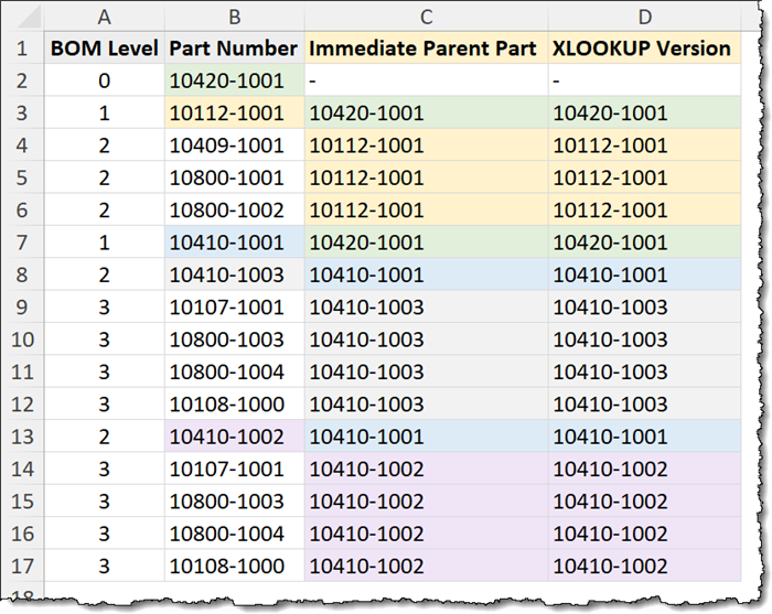
If we use the XLOOKUP function to solve the previous problem, the formula will look like the following:

Compared to the old-school LOOKUP with its confusing division process, XLOOKUP’s more elegant approach yields the same results.
Understanding the XLOOKUP Example
The XLOOKUP’s arguments (starting in cell D2) are as follows:
- A2-1 – This serves the same purpose: reduce the current BOM Level by 1.
- $A$2:A2 – The dynamically resizing lookup_vector.
- $B$2:B2 – The dynamically resizing results_vector.
- “-” – The text to display when no result is discovered.
- 0 – The match_mode. In this case, 0 equates to “exact match” mode.
- -1 – The search_mode. In this case, -1 equates to “search last-to-first” (e., bottom-up).
It’s that final argument that makes it work as desired.
Practice Workbook
Feel free to Download the Workbook HERE.

Featured Course
Master Excel Power Query – Beginner to Pro

Leila Gharani
I'm a 6x Microsoft MVP with over 15 years of experience implementing and professionals on Management Information Systems of different sizes and nature.
My background is Masters in Economics, Economist, Consultant, Oracle HFM Accounting Systems Expert, SAP BW Project Manager. My passion is teaching, experimenting and sharing. I am also addicted to learning and enjoy taking online courses on a variety of topics.


