Below is a list of commonly used Excel functions for Engineers:
- REPT
- TRIM
- LEN & SUBSTITUTE
- LEFT & RIGHT
- FIND & SEARCH
- LOOKUP
- IFERROR
- IF
As stated, these are not restricted to engineering uses; we can use these in hundreds of different non-engineering situations. But let’s pretend we’re engineers. It’s fun to pretend.
We start with a dataset that appears as follows:
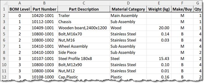
Column A contains a “Bill of Material” level (BOM Level), and Column B contains a Part Number.
The BOM Level represents a hierarchy of products. The “Trailer” at Level 0 is the parent to “Chassis” and “Wheel Assembly”. “Wheel Assembly” is the parent to “Side Piece” which is the parent to “Nut, M12”.
That’s a lot to remember, so let’s visualize this parent/child relationship between selected parts.
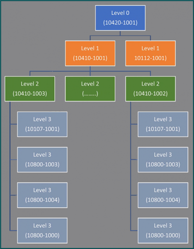
We also have information like:
- Material Category
- Weight
- Whether it was made or bought
- Quantity
Now let’s work on the data set.
Featured Course
Excel Essentials for the Real World

The REPT Function
The REPT function allows you to repeat a set of characters as many times as you want.
For our purposes, we want to use REPT to get indented part numbers. The indents will allow us to visualize our hierarchy more clearly.
To achieve this look manually, we’d have to copy/paste the part numbers into a new column, then add a series of indentations before each part number to achieve the desired indentation level.
This will take a lot of time, energy, and a high likelihood of inducing typographic errors.
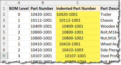
We can’t feed the REPT function an indentation instruction, but we can use three spaces to simulate an indentation. This is also a great way to achieve this look because we can easily increase or decrease the indentation by adjusting the number of spaces.
We’ll use the REPT function to add three spaces before the part number if it is a BOM Level “1”, six spaces if it is a BOM Level “2”, and nine spaces if it is a BOM Level “3”. Level “0” will not be indented.
We begin by inserting a new Column C and writing the following formula in cell C1.
=REPT(" " , 3 * A2) & B2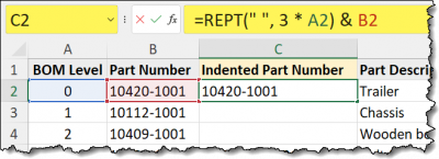
The REPT function multiplies the “3” by the BOM Level value then concatenates the part number to the end.

Featured Course
Power Excel Bundle

The TRIM Function
The TRIM function removes any leading or training redundant spaces from text. It also removes and redundant spaces from within the text.
If we were working with indented text like from the previous REPT example, but we needed a flat list of part numbers, we can write add a blank column to our data and write the following formula using the TRIM function:
=TRIM(B2)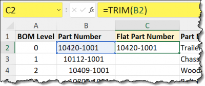
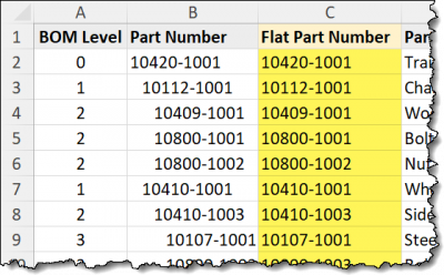
This produces a list of flattened part numbers having had all the leading spaces removed from the hierarchy.
The LEN and SUBSTITUTE Functions
The LEN function will return the number of characters in a text string while the SUBSTITUTE function will replace a character or string of characters with another character or string of characters.
If we were given a file where the hierarchy was displayed more like WBS (Work Breakdown Structure) codes, but we need the numbers as we’ve seen in earlier examples, we can write a formula to produce these numbers.
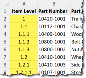
Each period starts a new level. An item with no periods is considered “Level 0” while an item with two periods is considered “Level 2”.
The logic for this substitution is as follows:
- Insert a new column (in this example, Column A).
- In cell A2, count the number of characters in the cell. This will be done using the LEN
- Replace all the “dots” with nothing. This will be done using the SUBSTITUTE function using two consecutive double quotes to symbolize nothing. Two continuous double quotes mean “empty text” to Excel. It’s like saying “show nothing”.
- Using the LEN function, count the number of remaining characters after the dots have been removed.
- Subtract the result from Step 4 from the result in Step 2.
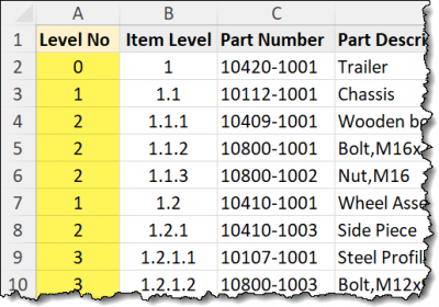
=LEN(B2) - LEN(SUBSTITUTE(B2, ".", "") )
Our results are as follows:
Featured Course
Unlock Excel VBA & Excel Macros

The LEFT, RIGHT and FIND Functions
The LEFT function extracts a set number of characters from a text string starting from the left side of the text.
We have been given a small table of Part Identities and quantities.
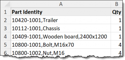
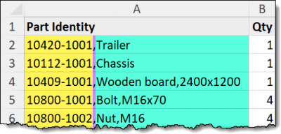
We need to separate the Part Number from the Description. These two elements are together in a single cell separated by a comma.
Finding the Part Numbers
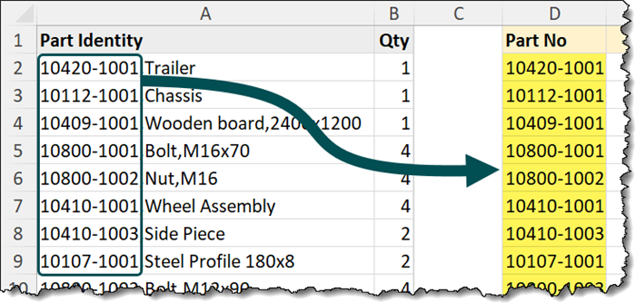
To separate the part numbers, we’ll start a new table (in Column D) and use the FIND function to locate the character position of the comma.
=FIND(",", A2)We can then use this value to tell the LEFT function how many characters to extract from the left of cell A2.
=LEFT(A2, FIND(",", A2) )We must deduct one from the value returned by FIND to not include the comma in the results.
=LEFT(A2, FIND(",", A2) - 1)
PRO TIP: The FIND function is case-sensitive. If you need to locate a character or string of text in a case-insensitive fashion, use the SEARCH function. The syntax and use are the same as the FIND function.
Finding the Descriptions
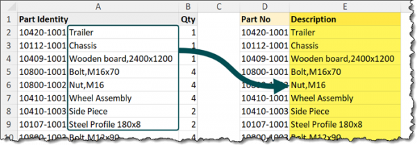
Because the descriptions are on the left end of the text in the Part Identity column, we will use the RIGHT function to extract a set number of characters from the right side of the text in Column A.
The key is to extract all characters after the comma.
We can use FIND to locate the comma as before. This will give us a count of all characters up to and including the comma.
=FIND(",", A2)The result of this FIND can be subtracted from the length of the entire text string to yield the number of characters to extract.
=LEN(A2) - FIND(",", A2)This value will be used by RIGHT to perform the extraction of the characters determined by LEN & FIND.
=RIGHT( A2, LEN(A2) - FIND(",", A2) )
The results are as follows:
The LOOKUP and IFERROR Functions
Discovering Data Using the LOOKUP Function
There will be many occasions where you need to discover an unknown piece of information based on a known piece of information.
An example may be something as simple as “How much does this chocolate chip cookie cost?”, or something more involved like “How many of this particular part number do we have in stock?”
Simple or involved, these questions can be solved using a lookup function.
Lookup functions have been part of Excel since its inception. Many methods have been developed over the years to discover related information. Functions like:
- LOOKUP
- VLOOKUP
- HLOOKUP
- INDEX/MATCH
- OFFSET
- XLOOKUP
Each of these functions has its strengths and weaknesses. Choosing the right one depends on the task at hand coupled with your knowledge and comfort level with each function.
The simplest (and oldest) lookup function is called LOOKUP. LOOKUP has lost favor over the years as more sophisticated, more capable functions have arrived on the scene. But that doesn’t mean it has lost its value.
LOOKUP lacks the pretentiousness of other functions, like INDEX/MATCH. Its charm is in its simplicity.
LOOKUP has the following syntax:
LOOKUP( lookup_value, lookup_vector, [result_vector] )In simpler terms:
- lookup_value – is the thing you know, like a part number, employee number, or cost code.
- lookup_vector – is the set of cells (a single row or column of cells) where the lookup_value may reside.
- [result_vector] – is the set of cells (a single row or column of cells) where the related item may reside.
For more detailed information and example on the use of LOOKUP, see the Microsoft Documentation for Excel’s LOOKUP function.
For our example, we want to discover the part number for the immediate parent of any child-level part number.
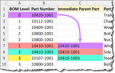
- Level 1’s parent is Level 0
- Level 2’s parent is Level 1
- Level 3’s parent is Level 2
To discover this, we can take the BOM Level of a child item (ex: Part Number “10410-1001” on row 7 has a BOM Level of “1”) and locate the nearest level “0” BOM Level that is above the current row.
Using the example above, the nearest BOM Level “0” is on row 2, Part Number “10420-1001”. (See the purple entries in the previous image.)
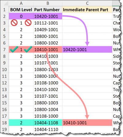
We can’t just write a lookup function that finds the first BOM Level that is 1 less than the current BOM Level.
At BOM Level “2”, there can be many level “1” entries above the current row. We must locate the closest (i.e., last listed) parent-level value that is above our current position.
We would need to ignore the level “1” item on row 3 and discover the level “1” item on row 7.
The formula we will use here is more sophisticated than most users are accustomed to. Perhaps a future post will break down the logic with greater specificity.
For now, we’ll just type it in as it relates to a lookup range in a LOOKUP function without diving into the details.
Starting in cell C2 of our example, we’ll write the following formula:
=LOOKUP(2, 1 / ($A$2:A2 = A2 - 1), $B$2:B2)The components are:
- lookup_value – 2
- lookup_vector – 1 / ($A$2:A2 = A2 – 1)
- [result_vector] – $B$2:B2

Hitting ENTER and filling the formula down the column produces the following results.
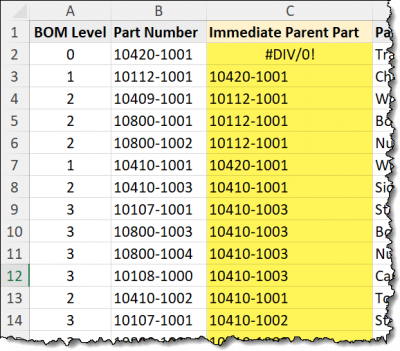
Observe the #DIV/0! error on row 2.

This is because BOM Level “0” has no parent-level item.
We can suppress this error message using the IFERROR function.
Displaying Custom Error Messages Using the IFERROR Function
Because many of the default Excel error messages are less than helpful to most users, we can trap the ugly error message and replace it with most anything we wish.
This is accomplished using the IFERROR function. IFERROR allows us to test a formula’s result. If the result is one of Excel’s built-in error messages, we can substitute the error with one of the following:
- Nothing (e., empty text)
- A text response
- A static value
- A different action via a formula
Since we know our BOM Level “0” items will return errors, we will trap the original errors and replace them with dashes.
=IFERROR(LOOKUP(2, 1 / ($A$2:A2 = A2 - 1), $B$2:B2), "-")
Now we have a more pleasing dash instead of an ugly error message.

Making Decisions Using the IF Function
IF functions allow you to ask a question then to act in one of two possible ways depending on the answer.
For our first example, we’ll perform a very simple IF that tests to see if the BOM Level is equal to a zero.
We’ll write the following in cell I2 and fill it down the column.
=IF(A2=0, "YES", "NO")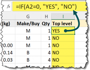
BONUS EXAMPLE
Let’s look at an example where we use three of the previously mentioned function in a single formula.
- IF
- IFERROR
- LOOOKUP
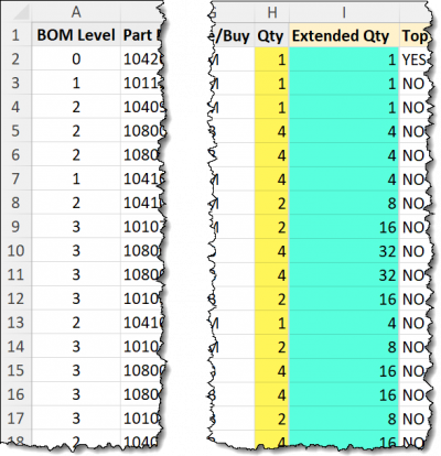
We’ll create a formula that calculates the quantity for each part at each level. The logic goes like this:
- If a BOM Level “1” has a quantity of 4, and
- its associated BOM Level “2” has a quantity of 2, and
- its associated BOM Level “3” has a quantity of 2, then
- each level is a multiple of its quantity against all previous quantities.
If we have a quantity of 4 at level “1”, and a quantity of 2 at level “2”, then we need 8 total at level “2”.
If we then need 8 at level “2”, and we have a quantity of 2 at level “3”, then we need 16 total at level “3”.
=IF(A2 = 0, H2, IFERROR(H2 * LOOKUP(2, 1 / ($A$1:A1 = (A2 - 1) ), $I$1:I1), "-") )
We’re using many of the same ideas presented earlier but in a more sophisticated way.
Practice Workbook
Feel free to Download the Workbook HERE.

Leila Gharani
I'm a 6x Microsoft MVP with over 15 years of experience implementing and professionals on Management Information Systems of different sizes and nature.
My background is Masters in Economics, Economist, Consultant, Oracle HFM Accounting Systems Expert, SAP BW Project Manager. My passion is teaching, experimenting and sharing. I am also addicted to learning and enjoy taking online courses on a variety of topics.


