This is a comparison of Excel from Microsoft 365 compared to Google Sheets.
The features highlighted here are presented from a high-level perspective and not discussed in step-by-step detail. Most of these features have been discussed in detail in previous posts. Links to the deep-dive posts will be supplied where possible.
#1 – XLOOKUP
XLOOKUP is a new lookup function that is intended to replace all other lookup functions, like VLOOKUP, HLOOKUP, and INDEX/MATCH.
XLOOKUP is much easier to use than any of the previous lookup methods while at the same time not burdened with any of the physical limitations or technical complications of other lookup strategies.
Perhaps the greatest advantage of XLOOKUP is the ability to return data from either the left or right side of the column being searched.
Another benefit of XLOOKUP is that it defaults to an exact match when performing a search.
Check out these posts to learn more about this amazing new function.
Left Lookup in Excel with XLOOKUP
#2 – Format as Table
Much of what we work with in Excel takes the form of tables; columns are categories and rows are records/transactions.
If we “upgrade” our table to an Excel Table, we unleash a slew of features that aid in design automation and formula creation.
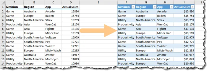
Below is a brief list of features available to us when using Excel Tables:
- Automatic color application to the table that is immune to corruption caused by sorting, filtering, adding, or deleting rows/columns.
- Automatic total row with a convenient dropdown to displaying common aggregations, like SUM, AVERAGE, COUNT, etc.
- Structured Reference syntax when creating formulas (ex: [Sales] $D$2:$D$500)
- Automatic heading promotion (freezing) when scrolling thru long tables.
- Automatic detection of new records (or removed records) to provide dynamic range references for formulas.
For more information on Excel Tables, visit the Overview of Excel Tables on Microsoft’s website.
#3 – Power Query
It can be argued that Power Query is perhaps the single best feature in Excel. It has been the topic of many posts here at XelPlus.
If you are unfamiliar with Power Query, it’s a feature that allows you to connect to dissimilar data sources (text files, web sites, Excel files, SharePoint, databases… the list is very extensive), combine the data, transform it to suit your needs, and produce a table or series of related tables in a data model.
These become the source material for things like charts and Pivot Tables.
It provides a user-friendly point-and-click interface for performing complex transformations of data without having to write complicated formulas or VBA macros.

The best part is, once created, the results of the query can be updated with new data with a single click of the mouse.
This feature is so extensive and powerful, I have an entire course devoted to its use.
Master Excel Power Query: Beginner to Advanced (including M)
To learn more about Power Query check out the following links.
Power Query Will Change Your Life
Power Excel (list of all related posts)
#4 – 3D Formulas
3D Formulas are a great way to create summary calculations based on data that spans multiple sheets.
Imagine having 12 sheets, January thru December, with sales for each month. In cell A1 of each sheet is the total of all sales for the respective month. Our objective is to add all the totals for the 12 months to get a yearly total.
What makes 3D Formulas so useful is that instead of referencing the same cell location for every sheet, in this case, it would be 12 references, we can reference the one cell while reducing the sheet references to a [StartSheet….FinishSheet] structure.
This…
=SUM(January!A1,February!A1,March!A1,April!A1,May!A1,June!A1,July!A1,August!A1,September!A1,October!A1,November!A1,December!A1)…becomes this…
=SUM(January:December!A1)We can add sheets to the workbook and have them automatically incorporate into the established calculation (provided certain requirements are met.)
For an in-depth guide to creating 3D Formulas, click here to read the full post.
#5 – Flash Fill
Excel’s Flash Fill is one of the greatest time-saving features when it comes to fixing data.
Flash Fill allows you to “fix” common data format issues like splitting text, merging text, date extraction, text replacement, formatting, and much, much more.
Flash Fill provides an alternative to learning many functions or features used to reshape data, such as:

To learn more about what Flash Fill can do to help you fix “bad data”, visit this post to read more.
#6 – The Data Model
If you need to create a Pivot Table (or Pivot Chart) that is based on data spread across multiple data tables, instead of combining the smaller tables into one large table, we can connect the smaller tables using Relationships.

Once we have created the relationships between our tables, we can view and manage the relationships in the Data Model.
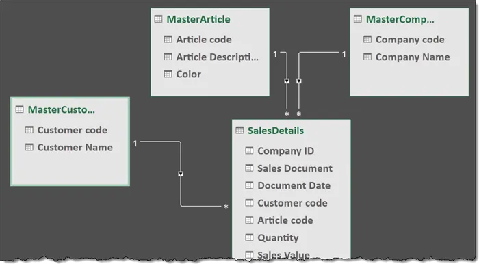
This allows us to create Pivot Tables that utilize elements from disparate tables without the need to create complex lookup functions to combine all of the smaller tables into a single, more cumbersome, and potentially memory-intensive table.
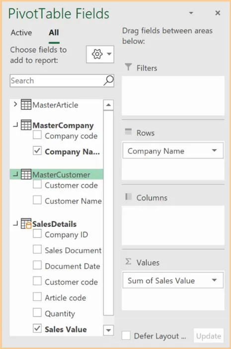
Visit the following Microsoft article to learn more about creating Excel Relationships and the Data Model.
#7 – Hash References
In Excel for Office 365, we can create what is known as a Hash References to reference a spilled range of formulas results.
A spilled range is where more than one result is returned from a single formula.
=FILTER(A2:C16, B2:B16 = G1, "Not Found")
The results of a spilled range can be used in a later calculation.
=SORT(F5#)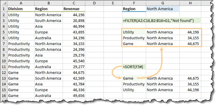
If the number of items returned from the spilled range changes (increases or decreases), the Hash References in later calculations will detect this change and adjust accordingly.
This keeps us from having to write complex formulas that determine the dimensions of the results.
Hash References are used extensively when using Dynamic Array functions. I have an entire course that revolves around Dynamic Array functions. If you haven’t used these new functions, they are worth your time to investigate. You will likely never go back to your old functions… unless you’re feeling nostalgic.
Excel Dynamic Arrays – New Functions and Calculation Methods
Excel Dynamic Arrays: Beginner to Expert (Office 365)
#8 – Flexible Charts
Because Excel has had time to mature over the past three decades, its feature sets when working with charts is quite extensive.
Using the built-in features along with the creative construction of your source data, you can create almost any visualization you need to represent your data.
You can create conditional bar charts.
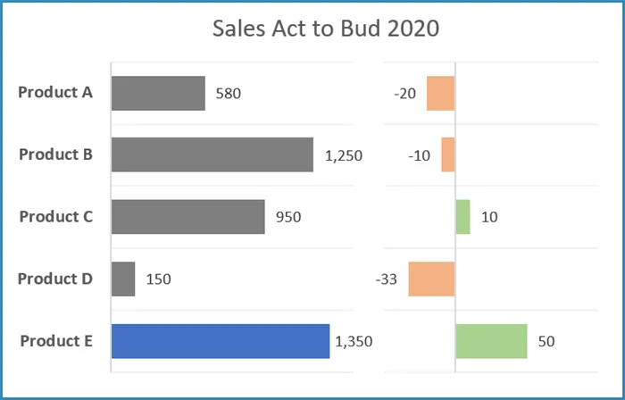
You can also get creative with infographics and create bar charts with icons like THIS or even a Gantt chart for your project tracking like THIS.
#9 – Go To Special
The Go To Special feature allows us to select all cells on a sheet based on the data in the cell or by a cell attribute.
We can select cells based on:
- Cells containing formulas
- Empty cells
- Cells using Conditional Formatting
- Cells using Data Validation
- Cells containing errors

We can access the Go To Special feature by pressing the F5 key then click the Special… button in the lower left of the Go To dialog box.
You can also activate the feature by selecting Home (tab) -> Editing (group) -> Find & Select -> Go To Special.

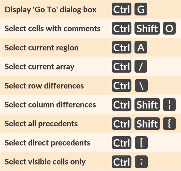
If you are into keyboard shortcuts, many of these Go To Special options can be invoked via a key combination on the keyboard.
#10 – Set Print Area
Excel allows you to select a range of cells and set it as the print area.

This ensures that only the area of interest is printed and not parts of the spreadsheet that may contain unrelated or sensitive data.
This range is saved as part of file data, meaning each time you open the workbook you can click Print and the system remembers what area is to be printed. You are not required to reselect the same area each time a printout is needed.
Click here to view my post on setting the print area along with other useful printing tips.
Bonus Features
There are many features that both Excel and Sheets offer, but Excel offers them with more features.
Slicers
When working with slicers in Excel, you receive visual feedback in the form of colors as to which slicer is selected, associated, non-associated, and not selected.
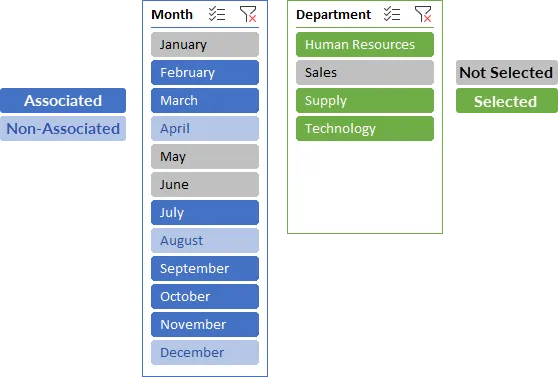
We also have a variety of cosmetic and behavioral treatments we can assign to the slicers.

To see a Slicer in action when using a Pivot Table and Pivot Chart, click here to read the post and watch the video.
Linking Shapes & Textboxes to Cell Contents
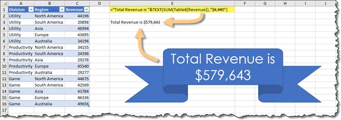
If you want to spice up your visuals with dynamic shapes, you can link a shape (or text box) to a cell. Whatever is being displayed in the cell can be automatically displayed on the shape.
A benefit of this feature is the ability to place cell results anywhere on the sheet or even a different sheet, regardless of the calculation’s cell address.
You can also apply any form of cosmetic treatment to the shape and text independent of the cell’s cosmetic settings.
Leila Gharani
I'm a 6x Microsoft MVP with over 15 years of experience implementing and professionals on Management Information Systems of different sizes and nature.
My background is Masters in Economics, Economist, Consultant, Oracle HFM Accounting Systems Expert, SAP BW Project Manager. My passion is teaching, experimenting and sharing. I am also addicted to learning and enjoy taking online courses on a variety of topics.


