Search for Features with Right-Click
It takes time to learn where all the Excel features are in the various ribbons. Excel possesses about forty different ribbon tabs, both standard and contextual, to house the hundreds of application features.
If a needed feature is being used for the first time (or hasn’t been used in some time), locating the feature can waste valuable time.
A fast way to locate any feature within the application is to right-click on any cell and use the “Search the menus” option located at the top of the right-click menu.
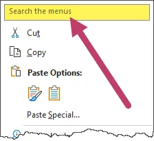
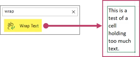
For example, say you want to wrap the text in a cell but can’t remember where the text-wrapping feature is located.
Right-click the cell with the text and type something like “wrap” in the search box.

This doesn’t just display the name of the feature that will serve your needs, rather it is the ACTUAL feature. You can click the listed feature and your needs have been met.
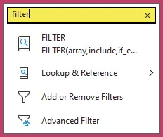
When presented with multiple actions in the search results, you can use the up and down arrow keys to navigate the list, then hit the spacebar or enter to invoke the needed action.
Featured Course
Excel Essentials for the Real World

Navigation Pane to locate Sheets and Objects
When working with workbooks that contain many sheets, often more than can be displayed at the bottom of the screen, it’s easy to lose track of where charts, shapes, tables, and other objects are located.
Locating and managing these assets is made easier when using the Navigation Pane.
To activate the Navigation Pane, click View (tab) – Show (group) – Navigation.

The right side of the screen displays a panel showing all of the sheets, charts, tables, and other objects contained in the workbook.
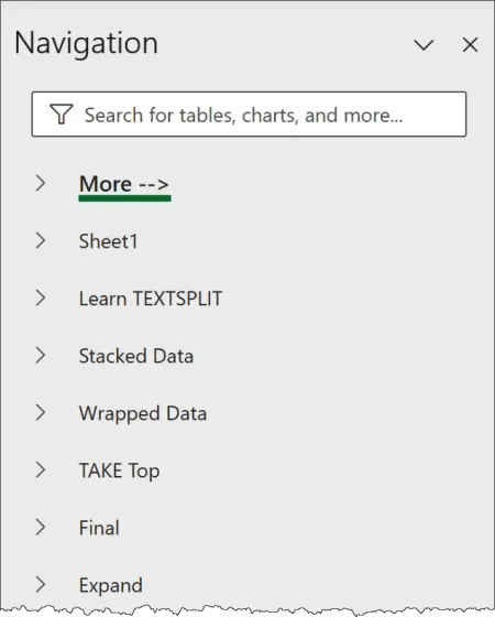
Right-clicking a sheet name will allow you to rename, hide, unhide, and delete the sheet.
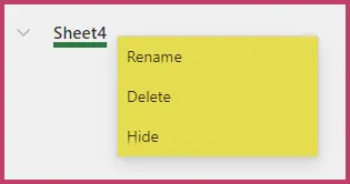
Hidden sheets will remain listed in the Navigation panel, but the names will appear in light gray to indicate a hidden state.
Clicking the Expand button to the left of a sheet’s name will display a list of all objects contained on the sheet. These can include (but are not limited to) charts, pictures, slicers, icons, tables, shapes, etc.
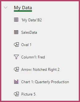
Clicking on a listed item will navigate you to that sheet and select the object in question.
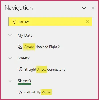
You can even leverage the search bar at the top of the Navigation panel to locate sheets or objects by name or type.
New Keyboard Shortcuts
Open the Power Query Editor
A super-fast way to open the Power Query Editor is to press the keyboard shortcut Alt-F12.

Copy and Paste as Values
To copy and then paste the cell results as static text (as opposed to the underlying formulas used to generate the results), you can do this quickly by following up the CTRL-C copy action with a CTRL-Shift-V instead of the normally used CTRL-V to paste.

This will perform the “Paste as Values” action normally accessed from a right-click, Paste Special menu.
Featured Course
Automate With Power Query – Recipes to solve business data challenges

Automate Tasks with Office Scripts
You may have noticed in later versions of Excel a new tab named Automate. It groups Excel’s newer automation features.

The Automate tab allows you to create scripts that will run on Excel for Desktops as well as Excel for the Web.
For example, suppose you need to make a chart based on data where the chart has the same consistent look and type.
With the Automate tab and Office Scripts, this can be performed in just a few clicks.
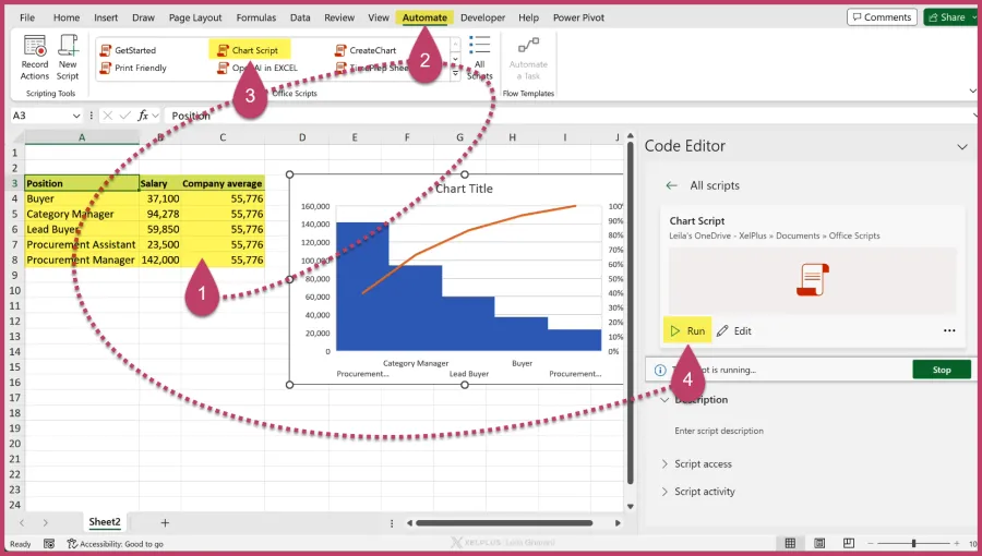
- Highlight the data to be charted
- Click the Automate tab
- Click “Chart Script” to activate the script created to make charts
- Click the Run button to execute the script
I have several videos for you that provide detailed demonstrations, examples, and instructions for creating, executing, and managing Office Scripts. Check these links below.
🔗Introduction to Office Scripts
🔗How to Use Office Scripts with Power Automate
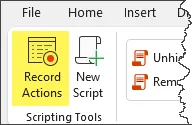
You don’t have to be a master coder to create Office Scripts. The Automate tab provides access to a script recorder labeled “Record Actions” that will write the code for you based on the buttons clicked and typed data.
Value Preview Tooltip to Evaluate Formulas in Part or Whole
If you are troubleshooting a formula error and can’t figure out where things went awry, a common trick is to highlight part of a formula in the Formula Bar and press the F9 key.
This will replace the highlighted section with the result that the section calculates.
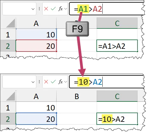
This can be dangerous as the F9 action will alter the formula from a dynamic calculation to a static value. Users must be mindful to hit the ESC key to return the formula to its original dynamic state.
To eliminate that danger, and make the process easier, you can use the Formula Bar to highlight portions (or all) of a formula, then observe the automatic tooltip that appears to see what that portion of the formula works out to.
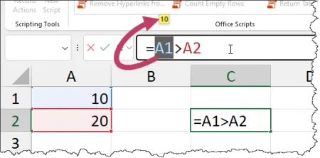
You can select references, functions, parameters within a function, or even the entire formula.
There’s no longer a need to press F9 and run the risk of corrupting the formula.
If you select a part of the formula that can’t be evaluated, you won’t see a tooltip.
Featured Course
Master NEW Excel Functions in Office 365 & Office 2021

Use Dynamic Array Results in Power Query
Historically, Dynamic Array results could not be used as a data source in Power Query.
That’s not to say that the results couldn’t be brought into Power Query, it’s that Power Query would fail to properly recognize the source data if the results were to expand beyond the originally selected cell range.
That issue has now been rectified with this new feature in Excel 365.
To bring the results of a Dynamic Array formula into Power Query, select the single cell that holds the formula, then click Data (tab) – Get & Transform Data (group) – From Table/Range.
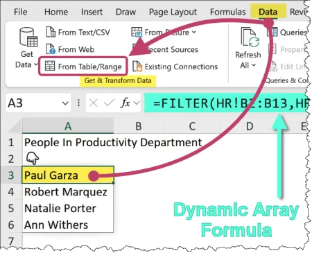
This brings the Dynamic Array results into Power Query and names the query “FromArray_X” (“X” being the instance number of imported arrays.)
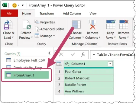
If the results of the Dynamic Array formula change, a refresh of the query will reflect the new formula results.
Use Dynamic Array Results as a Chart Source
In the same vein as Power Query, Excel charts could not utilize the changing range of Dynamic Array output as a data source. Or, at least, it required a lot of effort and complex formulas to set it up. It became much simpler.
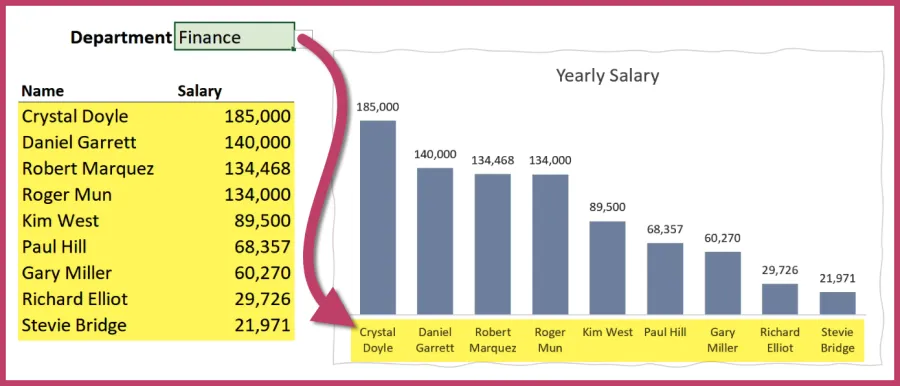
Charts can now use this output and automatically update when said output changes.
For example, we have used a series of Dynamic Array functions to create the output seen in cell E5.

Next, we have created a chart based on the Dynamic Array output to show the yearly salary for all employees in the “Procurement” department.
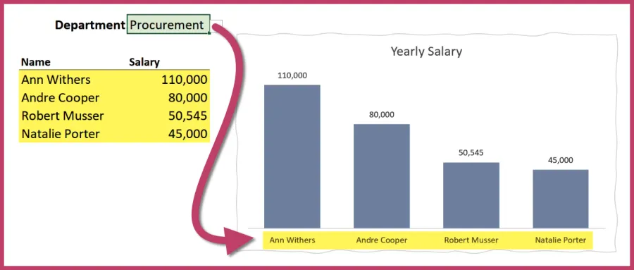
If the department dropdown is changed to “Finance”, the chart updates to reflect the new Dynamic Array output.
I have a separate video that demonstrates the process of using Dynamic Array output as a chart data source:
📺Effortlessly Create Dynamic Charts in Excel: New Feature Alert!
Cheat Sheet
Download the handy Cheat Sheet with all the exciting new features:
Featured Course
Black Belt Excel Package

Leila Gharani
I'm a 6x Microsoft MVP with over 15 years of experience implementing and professionals on Management Information Systems of different sizes and nature.
My background is Masters in Economics, Economist, Consultant, Oracle HFM Accounting Systems Expert, SAP BW Project Manager. My passion is teaching, experimenting and sharing. I am also addicted to learning and enjoy taking online courses on a variety of topics.


