New Features in Excel 2021
Every new release of Office brings with it new Excel functions.
In Office 2019 we were introduced to new functions, such as:
- MAXIFS
- MINIFS
- IFS
- TEXTJOIN
- CONCAT
- SWITCH
If you are an Office 2016 user and are upgrading directly to Office 2021, check out these “new to you” functions.
For Office 2019 users upgrading to Office 2021, we have a new batch of functions that are about to change your Excel life forever. These functions include:
- XLOOKUP
- XMATCH
- UNIQUE
- SORT
- SORTBY
- SEQUENCE
- RANDARRAY
- FILTER
- LET
Many of these new functions are referred to as Dynamic Array functions.
Dynamic Array functions have many features that regular functions lack, such as the ability to “spill” many results from a single formula, as well as mitigate (in many cases) the need for changing a relative reference to an absolute reference.
For a more in-depth explanation of these functions check out these links:
Excel 365 Functions for 2021
Excel’s New LET Function
Excel XLOOKUP Explained
Excel FILTER Function
Yearly Calendar in Excel with Formula
With these new functions, you’ll spend far less time trying to create complex, multi-layered functions to accomplish tasks.
For example, imagine trying to display all the employees in a list that belong to the “Sales” department.
In Excel 2019, the formula would look something like this:

In Excel 2021, that same activity can be accomplished using this:

Let’s look at some of these new functions.
Featured Course
Master NEW Excel Functions in Office 365 & Office 2021

The UNIQUE Function
The UNIQUE function allows you to return a list of unique values from another list.
The function is simple; point to the list of existing data.
If we have a list of Departments and we want to see a “one of each” list, we can write a formula like the following.
=UNIQUE(A2:A13)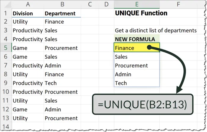
Earlier versions of Excel required writing a formula like this:

Unless you’re the type that just REALLY loves a challenge, I’m certain you’ll prefer the new technique.
Bonus Feature
If we were to use the longer, older formula to create our unique list of Departments, we would be responsible for repeating the formula down the column for as many departments as we expect to be returned.
With the new Dynamic Array functions, the results automatically “spill” into the needed cells. No need to use a Fill Series or pesky CTRL-Shift-Enter key sequence.
The FILTER Function
Unlike the VLOOKUP function which can only return a single value of the first encountered match in a list, the FILTER function can return entire rows worth of data for every matching item in a list.
Suppose we need to return a list of employee names based on a selected department.
The FILTER function is simple: where’s the list of items to search, then what is the search criteria?
In this example, we want to return every name in column B that matches the selection in a dropdown (cell F3) to a list of departments in column A.
The formula would appear as follows:
=FILTER(B2:B21, A2:A21 = F3, “”)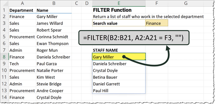
The last argument that contains two double-quote marks is to tell FILTER what to display if no results are discovered. In this case, display nothing.
The older way of accomplishing this act looked like so:

The worst part is that’s not the only formula you had to write. There were supporting formulas that had to be created to assist this formula.
Most users would rather have a root canal than deal with this problem.
The SORT Function
This is one the simplest yet most useful of the new functions.
If you want to derive a sorted list of items, just place the list in the function.
=SORT(A2:A13)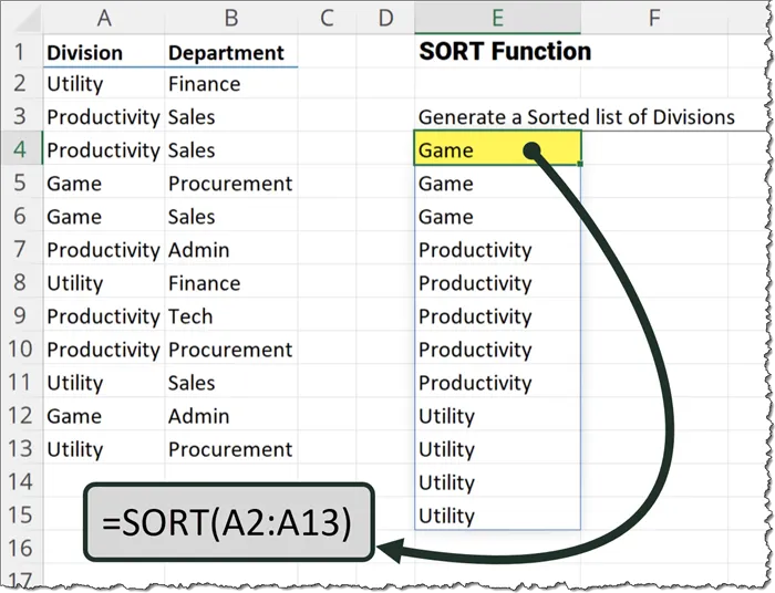
The default sort order is “ascending”, but if you want a “descending” list, you can add an argument to the formula.
=SORT(A2:A13, , -1)What makes the new SORT function so versatile is when you combine it with other functions like the UNIQUE function or FILTER function.
This will take the results of those functions and sort them by whatever method you desire.
=SORT(UNIQUE(A2:A13) )
Featured Course
Master Excel Power Query – Beginner to Pro

The SORTBY Function
This new function allows you to sort one list based on the criteria of another list.
Suppose we need to create a list of all employee names, but we want the list sorted by those employees’ yearly salaries in descending order (-1).
The SORTBY allows you to point to one list (the list that needs to be sorted) then to a second list that serves as the sort criteria.
=SORTBY(A2:A11, B2:B11, -1)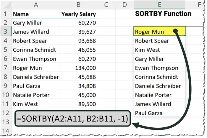
The XLOOKUP Function
The XLOOKUP function is the lookup function to replace all lookup functions.
If you have used VLOOKUP, HLOOKUP, or struggled with INDEX/MATCH, this is the answer to your lookup prayers.
XLOOKUP can locate items in a table that reside to the right or the left of your lookup column. This means the column order of your table is no longer a factor.
XLOOKUP possesses many other features such as:
- The ability to display a custom message if no items are found
- The ability to perform exact match searches or return the closest/smallest result or the closest/largest result
- Search from the beginning of a list or start the search from the end of the list.
The below example locates the selected employee name (cell G6) in a list of names (B2:B14) and returns the employee’s salary (C2:C14).
=XLOOKUP(G5, B2:B14, C2:C14)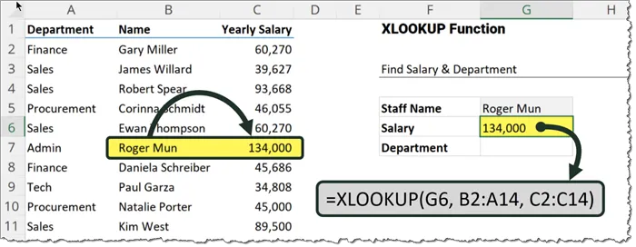
If we need to discover the Departments for the selected employee, this is not an issue for XLOOKUP even though the Department column is to the left of the search column.
=XLOOKUP(G6, B2:B14, A2:A14)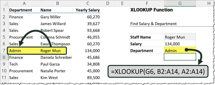
The old way to “look to the left” was to use an INDEX/MATCH combination. This is not too difficult, but many users struggle with the concepts.
Plus, you’d have to incorporate an IFERROR function to deal with situations where no items were found.

The XLOOKUP that incorporates error checking would look like so:

The XMATCH Function
Like the older MATCH function, the XMATCH function returns the relative position of an item in a list.
What makes the XMATCH function more powerful are the ability to:
- Default to an exact match mode
- Return the first encountered match starting from the top of the list
- Return the first encountered match starting from the bottom of the list
- Perform wildcard matches
- Work with sorted or unsorted lists
The SEQUENCE Function
The SEQUENCE function generates a list of numbers in an order and sequence that you want.
This can be a list of numbers as simple as “1, 2, 3, …” or more complex as in a two-dimensional array of sequential fractions.
SEQUENCE allows you to define a number of rows and/or columns, a start value, and value by which to increment.
A simple “1, 2, 3, …” list would be written with the following formula.
=SEQUENCE(10, 1, 1, 1)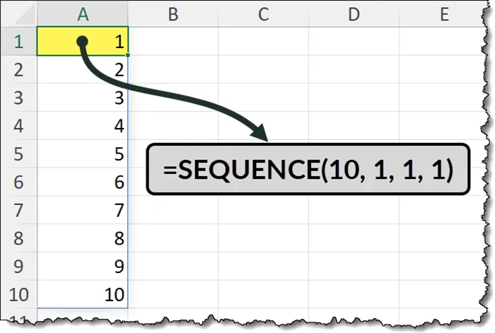
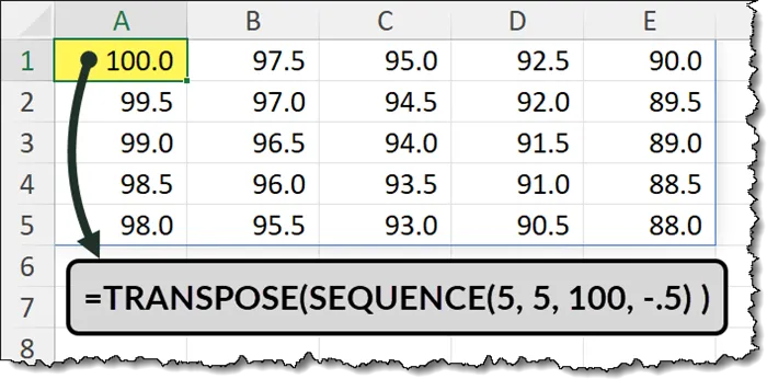
A 5 by 5 array of fractions (decrementing by one-half) would appear as follows.
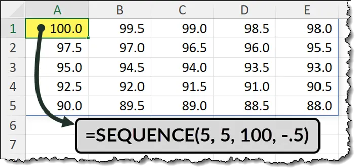
If you wanted the results to display vertically instead of horizontally, you can nest the above formula within a TRANSPOSE function.
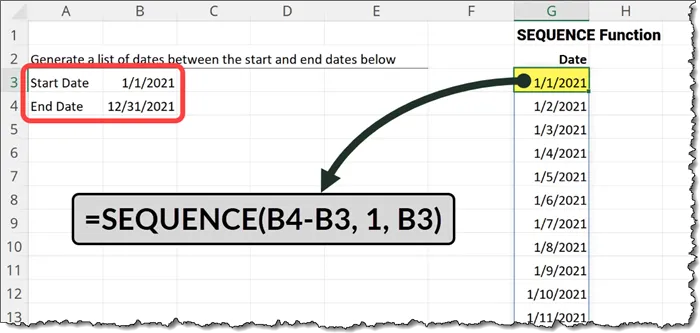
A great use of SEQUENCE is to generate lists of dates.
For example, since dates are just numbers, it’s easy to list dates starting from a start date (cell B3) and list all dates till the end date (cell B4). The number of rows in the sequence is the difference between the end date and the start date (B4 – B3).
=SEQUENCE(B4-B3, 1, B3)NOTE: The default step/increment is 1, so we can leave it out of the above formula and make a shorter formula.
The RANDARRAY Function
The RANDARRAY function creates one or two-dimensional arrays of random fractions or whole numbers.
This is like the older RAND and RANDBETWEEN functions, but with greater flexibility.
The arguments are:
RANDARRAY([Rows], [Columns], [Min], [Max], [Integers])Here are some examples:
- Create an array of random fractions less than 1 in a 10 row by 1 column array.
= RANDARRAY(10, 1)- Create an array of random fractions less than 1 in a 1 row by 10 column array.
= RANDARRAY(1, 10)- Create an array of random fractions less than 1 in a 5 row by 5 column array.
= RANDARRAY(5, 5)- Create an array of random fractions between 10 and 120 in a 5 row by 5 column array.
= RANDARRAY(5, 5, 10, 120)- Create an array of random whole numbers between 10 and 120 in a 5 row by 5 column array.
= RANDARRAY(5, 5, 10, 120, TRUE)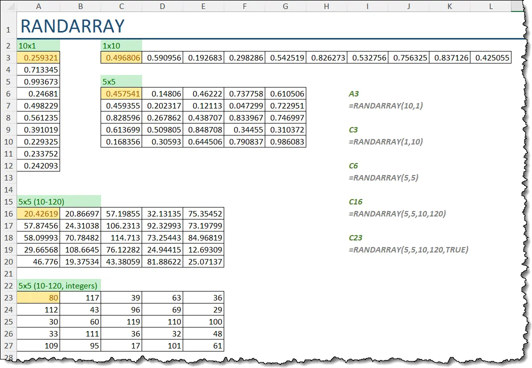
(Click for larger image)
PRO TIP: Press the F9 key to regenerate the random values.
The LET Function
The LET function allows you to define names for portions of your formula that may repeat several times within the same formula.
There are several advantages to using LET in these types of situations:
- The repeating portion only needs to be written once.
- The calculation need only occur once, while the result can be reused as many times as needed in the formula. This can be a great boon to performance.
- Maintenance on the formula is easier since it only needs to occur once.
The repeating formula is given a nice, user-friendly name that is referenced in the actual calculation.
This is like giving a cell a named range, like “Discount”, and using that name in a formula instead of an ugly cell reference, like $K$19.
For example, if we were to calculate a variance that is plus or minus 10% between actual and budgeted revenue, we could write the following formula.
IF(ABS(B2/C2 – 1) > 10%, B2/C2 – 1, “”)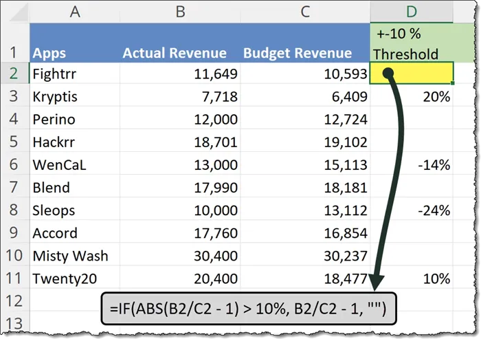
Notice how the calculation “B2/C2 – 1” is performed twice for every row in the table.
Writing this same formula using the LET function, we can write the formula once and give it a name, like “var”, then use that name in every original location.
=LET(“var”, B2/C2 – 1, IF(ABS(var) > 10%, var, “”) )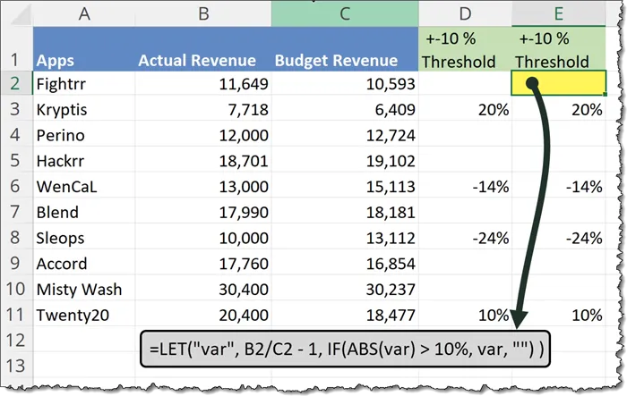
I know it looks like our formula just got more complicated, but if you look closely you’ll see that the only additional part is the naming of the formula (“var” as equal to the formula “B2/C2 – 1”).
The second half of the formula is the same as the first but only using the name “var” wherever the original formula occurred.
Additional New Excel Features
Using “Sheet View” During Collaboration
When collaborating with others online where more than one user is working in the same document, filtering a table to aid in your mission will apply the same filter to the other online viewers of the file.
Needless to say, this can start a mini filter war between the participants.
To create a duplicate view of the sheet that allows for individualized filters (i.e., filters only you see), you can create a new Sheet View.
The Sheet View features are located on the View tab.
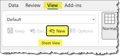
Views can be named and saved for later reuse.
This is a great way to “bookmark” the sheet when you have filtered or grouped data to tell a specific story.
NOTE: Sheet views are currently limited to Excel 2007 or later files stored in OneDrive, OneDrive for Business, and SharePoint.
Featured Course
Master Excel Power Pivot & DAX (Beginner to Pro)

Never Lose Your Data with AutoSave
AutoSave is a new feature available in Excel, Word, and PowerPoint for Microsoft 365 subscribers that saves your file automatically, every few seconds, as you work.
AutoSave is enabled by default in Microsoft 365 when a file is stored on OneDrive, OneDrive for Business, or SharePoint Online.

This provides peace of mind if your computer is prone to crashes or power loss.
The feature can be toggled on or off at your discretion. This is helpful if you want to experiment with something in your file, but do not wish to save the results of the experiment.
Set Colors with HEX Codes
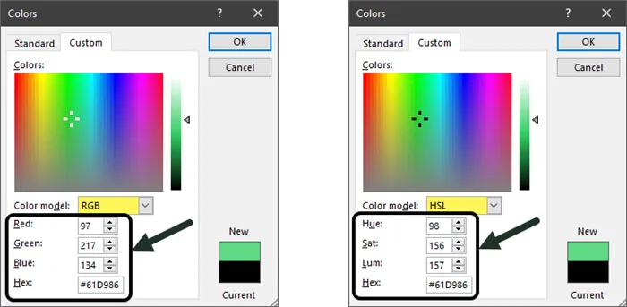
When applying colors to text or objects, you are no longer restricted to RGB codes. You can now utilize HEX, and HSL codes.
Icons & Illustrations
We now have access to a plethora of icons and images to enhance our documents.

(Click for larger image)
These even include 3D models which can be positioned and viewed from any angle or zoom factor. Some are even animated. (Check out the running cross-sectional jet engine. WAY cool!)
PowerPoint Recording Tools
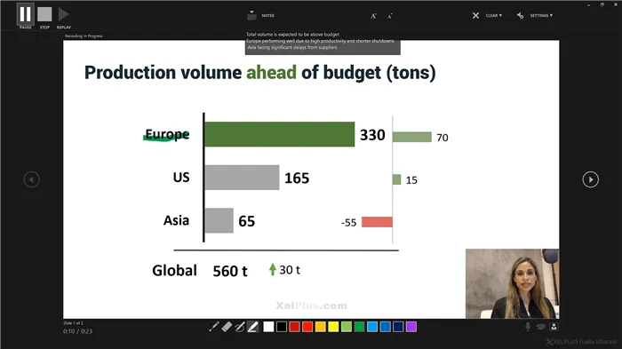
PowerPoint now includes the following screen recording enhancements:
- A countdown timer to indicate when recording has begun.
- Easy to access and understand annotation tools.
- Thumbnail view of Picture-in-Picture webcam recording.
- Viewable slide notes that act as a teleprompter but are not seen by the recorder.
Word Immersive Reader Improvements
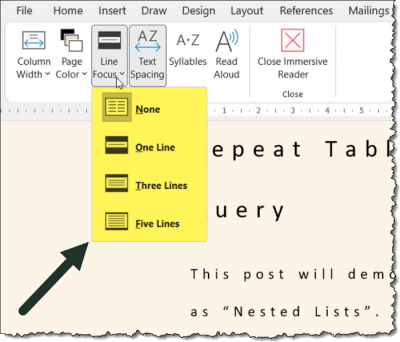
The new Immersive Reader allows you to decide how many lines you want to focus on at a time.
Improved Instant Search for Outlook
In my opinion, the most improved feature in Outlook is the Instant Search feature.
This allows you to search for items based on date, sender, attachments, status, etc.
For a full breakdown of the new Instant Search feature, check out this link.
Outlook Search the Right Way
Leila Gharani
I'm a 6x Microsoft MVP with over 15 years of experience implementing and professionals on Management Information Systems of different sizes and nature.
My background is Masters in Economics, Economist, Consultant, Oracle HFM Accounting Systems Expert, SAP BW Project Manager. My passion is teaching, experimenting and sharing. I am also addicted to learning and enjoy taking online courses on a variety of topics.


