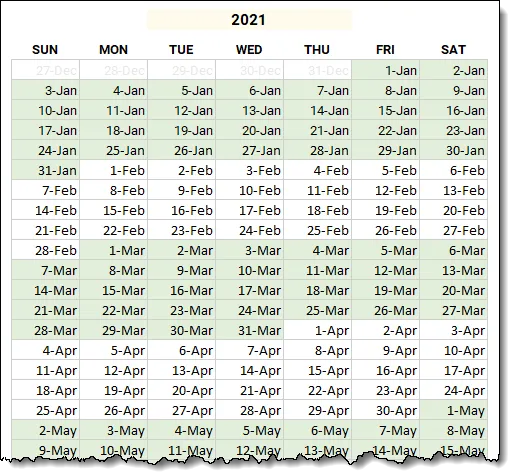
To make our interactive yearly calendar as seen above, we will take advantage of one of the new Excel Dynamic Array functions called SEQUENCE.
User Input and Formula Output
The goal is to have the user type a year in a cell, such as D2, and have the SEQUENCE function generate all the calendar dates for that year, structured in a 7-day by 54-week table.
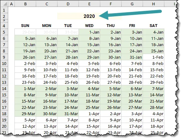
NOTE: We require a 54-week table because of an oddity that occurs every 28 years. Using the year 2000 as an easy start, the month of July has 6 weeks. This adds an extra week to the more common 53-week year. Every 28 years before and after the year 2000 have this same behavior.
Building the Table
We start by creating the headers that will describe the day-of-the-week columns.
Enter the weekday names in cells B4 through H4.

You can format the headers as you please (ex: bold and centered with colored, thick underline).

Writing the Magic Formula
The driving force behind this formula is the SEQUENCE function.
To understand the SEQUENCE function, the syntax is as follows (parameters in brackets are optional):
SEQUENCE(rows, [columns], [start], [stop])- rows – is the number of rows to return.
- [columns] – is the number of columns to return. (the default is 1)
- [start] – is the first number in the sequence. (the default is 1)
- [step] – is the amount to increment each subsequent value in the array. (the default is 1)
Let’s break this down into its constituent parts.
ROWS – The number of rows is easy… 54 (see the above note if you missed that part.)
=SEQUENCE(54,COLUMNS – The number of columns for our week is 7.
=SEQUENCE(54, 7,Here’s where it gets trickier.
START – The first number (i.e. date) must be a date that occurs on a Sunday. This does NOT necessarily mean the first Sunday in the selected year, as January 1st does not always fall on a Sunday. In those cases, the first Sunday in our table will be a date from the previous year.

To keep things simple, we will occupy this argument with a “1”. We’ll make it dynamic later.
=SEQUENCE(54, 7, 1STEP – This is the value by which all subsequent dates will be incremented. Since we want every day in the year, we will use a STEP value of “1”.
=SEQUENCE(54, 7, 1, 1)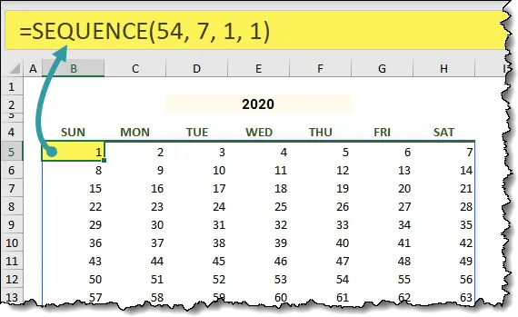
Turning Numbers Into Dates
We need a sequence of dates, not numbers. We can substitute a date in the third argument (START). This way, the numbers start at that defined day.
Let’s start with a static date of January 1, 2020. We will use the DATE function to generate the date using the user-supplied year in cell D2.
DATE(D2, 1, 1)When folded into the existing SEQUENCE function, the updated formula appears as follows:
=SEQUENCE(54, 7, DATE(D2, 1, 1), 1)The results are displayed as unformatted numbers.
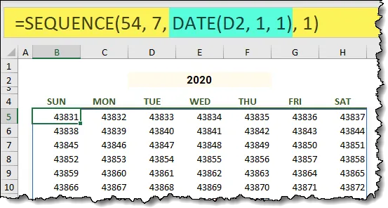
Selecting the cells where we expect to see results, format the cells with a date style such as “d-mmm”.
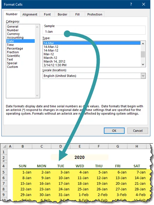
The “Tricky” Part
The tricky part falls in that third argument; START.
We need to have the first number represent the first Sunday of the first week in the selected year.
Step 1: Determine the weekday of January 1 of the selected year
We know that the DATE function will generate our “first day of the year” date. We can use the WEEKDAY function to determine the “day of the week” number of that date.
When we fold that logic into the existing DATE function, we see the following:
WEEKDAY(DATE(D2, 1, 1) )This yields a number between 1 and 7.
This would result in a 4, meaning “Wednesday”.

Step 2: Find the difference between “Sunday” and “January 1”
We can use the value derived by the WEEKDAY function to “roll back” a set number of days from the date generated by the DATE function.
DATE(D2, 1, 1) - WEEKDAY(DATE(D2, 1, 1) )The updated SEQUENCE function appears as follows:
=SEQUENCE(54, 7, DATE(D2, 1, 1) - WEEKDAY(DATE(D2, 1, 1) ), 1)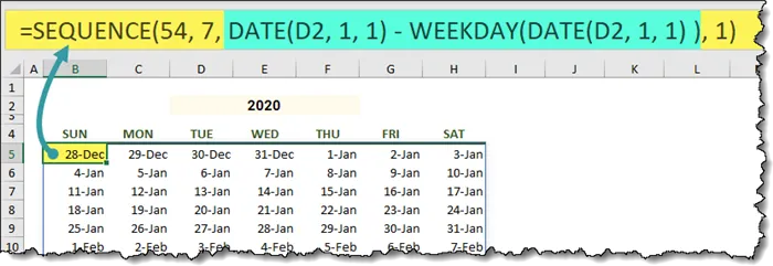
The problem with this is we have rolled back one day too far.
We need to adjust the DATE/WEEKDAY logic to add one day to the result.
=SEQUENCE(54, 7, DATE(D2, 1, 1) - WEEKDAY(DATE(D2, 1, 1) ) + 1, 1)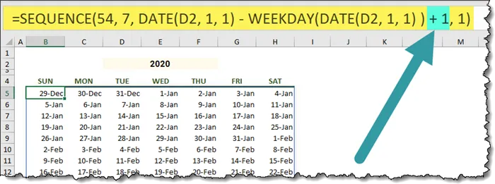
Now, let’s apply some formatting to make the calendar easier to read.
Add Borders to the Calendar
To give the calendar a nice grid-style, we will add borders to all of the cells that we anticipate dates to occupy.
Select the results range and apply a medium-gray border to all interior and exterior cell walls.
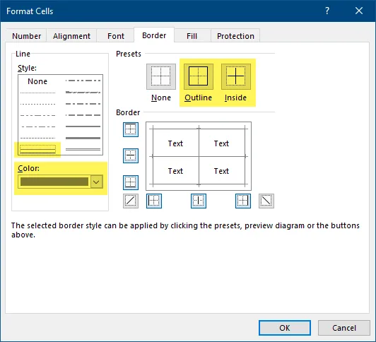
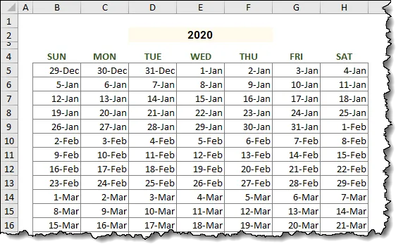
The results of the borders appear as follows:
Faded Font for “Out of Year” Dates
To make it obvious which years are not part of the selected year, we will apply a light-gray color to any “out-of-year” dates. This will be accomplished using Conditional Formatting.
The logic is simple: of the year of the cell date is not in the current year, apply a light-gray font color to the cell.
- Select the cells holding dates.
- Select Home -> Conditional Formatting -> New Rule.
- Select “Use a formula to determine which cells to format”.
- Use the custom formula below.
=$D$2 <> YEAR(B5)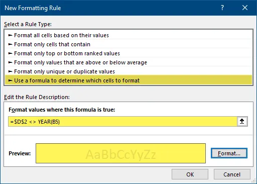
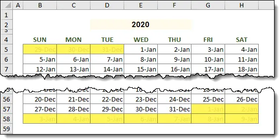
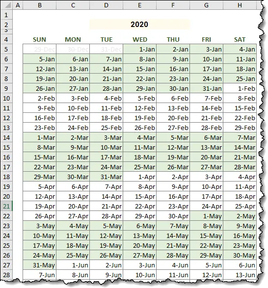
The result is a calendar that fades the non-applicable days.
Shading Every-Other Month
The final touch is to have the odd-numbered months shaded with a pale-green fill color.
To accomplish this, we will perform the following logic steps:
- Extract the month from the date using the MONTH
- Divide the month number by 2 and retain only the remainder. This is performed using the MOD
- If the remainder is 1 (seen by Excel as “TRUE”), we apply the cell shading. If the remainder is 0, the cell is left to its original color.
NOTE: Excel treats 0 (zero) as “FALSE” and any other non-zero number as “TRUE”.
To implement the logic, perform the following steps:
- Select the cells holding dates.
- Select Home -> Conditional Formatting -> New Rule.
- Select “Use a formula to determine which cells to format”.
- Use the custom formula below.
=MOD(MONTH(B5), 2)If you are unfamiliar with the MOD function, click here to see a more in-depth video-post about the MOD function.
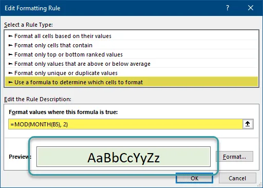
The result is a calendar with alternating month shades.
Tweak the Shading Rule
In those cases where you do not have a 54-week year, the shading at the bottom of the calendar looks a bit extraneous.
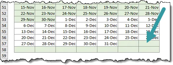
This is easily fixed by reordering the Conditional Formatting rules.
Perform the following steps:
- Click any cell in the calendar table.
- Select Home -> Conditional Formatting -> Manage Rules.
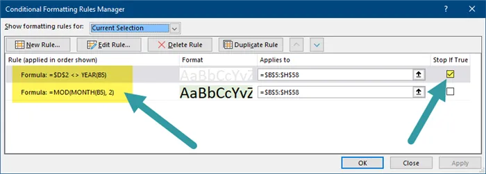
- In the Manage Rules dialog box, reorder the rules so the “out-of-year” rule is first and the shading rule is second.
- Place a checkmark in the “Stop if True” option of the first rule.
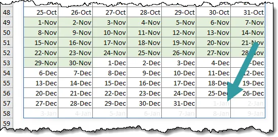
The results are as follows:
Generating a Single Month Calendar
Thanks to a viewer that goes by the name “CR GR0912”, they have developed a formula that allows the user to define a month and year which is then used to generate a single month calendar.
To generate a calendar for a specified year and month, the following formula can be used:
=LET(m, A2, y, B2, d, 1, dw, {"Sun","Mon","Tue","Wed","Thu","Fri","Sat"}, sq, SEQUENCE(8), dt, DATE(y, m, d), fd, DATE(y, m, 1), wd, WEEKDAY(fd), dts, SEQUENCE(8, 7, fd-wd-13), arr, IF(MONTH(dts)=m, TEXT(dts, "d"), ""), r1w, TEXT(dt, "mmm yyy"), r2w, REPT(dw, SEQUENCE(2, , 1, 0) ), IFS(SEQUENCE(8, 7)=3, r1w, sq=2, r2w, TRUE, arr) )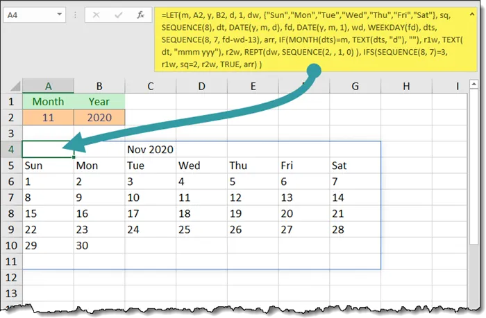
By placing a month number in cell A2 and a year in cell B2 we can generate the following calendar.
If you need to have your calendar start on a Monday instead of a Sunday, you can use the below version of the code:
=LET(m, A2, y, B2, d, 1, dw, {"Mon","Tue","Wed","Thu","Fri","Sat","Sun"}, sq, SEQUENCE(8), dt, DATE(y, m, d), fd, DATE(y, m, 1), wd, WEEKDAY(fd, 2), dts, SEQUENCE(8, 7, fd-wd-13), arr, IF(MONTH(dts)=m, TEXT(dts, "d"), ""), r1w, TEXT(dt, "mmm yyy"), r2w, REPT(dw, SEQUENCE(2, , 1, 0) ), IFS(SEQUENCE(8, 7)=3, r1w, sq=2, r2w, TRUE, arr) )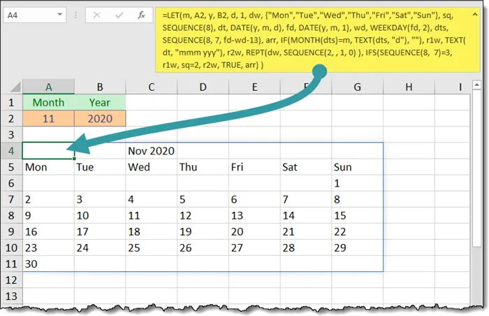
Learn More About Dynamic Array Functions
You have just witnessed the awesome power of a Dynamic Array function. Having a single function create the foundation for something as vexing as a dynamic calendar template should excite your brain in new and exciting ways.
If you’d like to see more examples using other fantastic Dynamic Array functions, click here to see my Dynamic Arrays playlist and consider enrolling in my Dynamic Arrays course.
Practice Workbook
Feel free to Download the Workbook HERE.

Leila Gharani
I'm a 6x Microsoft MVP with over 15 years of experience implementing and professionals on Management Information Systems of different sizes and nature.
My background is Masters in Economics, Economist, Consultant, Oracle HFM Accounting Systems Expert, SAP BW Project Manager. My passion is teaching, experimenting and sharing. I am also addicted to learning and enjoy taking online courses on a variety of topics.


