To understand the FILTER function, the syntax is as follows (parameters in brackets are optional):
FILTER(array, include, [if_empty])
- array – is the range or array you want to be included in the result. This can be the entire data set or part of the original data set.
- include – is the test you are performing on each record in the data set. This is the engine that moves the FILTER function forward. Here is where you define the criteria for included versus excluded records.
The logic will resemble the test portion of an IF function; we select a range of cells and compare each item in the range to a defined value (ex: B8:B40=E6, where column B is the data and cell E6 is what the data is being compared against.) Any record that results in a TRUE statement will be included in the results. Any record that results in a FALSE statement will be excluded from the results. - [if_empty] – defines what is to be displayed if no records match the include test (ex: “No Data”). Although this argument is optional, if it is not defined, and no data is returned from the include test, a #CALC! error will be displayed.
Let’s look at some examples of the FILTER function in action.
EXAMPLE #1 – Filter by Region
- Begin by opening the START file and select the FILTER
Starting the results in cell F7, we wish to display all the records from our data set (cells A5:C20) that match the region selection defined in cell G5 (i.e. “Asia”).
This will be like performing a VLOOKUP, but instead of returning a single value, we will return all the information about each qualifying record.
- Select cell G5 and enter the region “Asia” as the comparison value.
- Select cell F7 and enter the following FILTER formula:
=FILTER(A6:C20, B6:B20=G5)
The formula spills and returns all the information from each record where the region matches cell G5 (“Asia”).
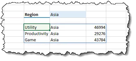
The formatting of the revenue does not carry over from the original data, so we need to fix that for the results list.
- Select cells H7:H9 and apply a Comma style with no decimal places. (NOTE: It is a good idea to format all the cells where you expect the list to spill to; even if you are not currently using those cells.)
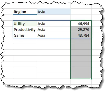
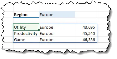
- Test the automatic updating of the formula by changing the region in cell G5 from “Asia” to “Europe”.
If we leave cell G5 empty or enter a region that does not exist in the data, the #CALC! error message is displayed.
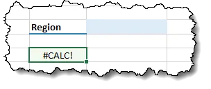
To overcome the error, in other words, replace it with something more user-friendly, we will update our formula to utilize the 3rd optional argument.
- Select cell F7 and enter the following FILTER formula:
=FILTER(A6:C20, B6:B20=G5, “Not Found”)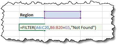
To make the changing of the regions easier for the user, we can incorporate a Data Validation drop-down list in cell G5. (NOTE: This can be done with greater power using spill ranges in drop-downs, but we go “old school” for now. Spill range drop-downs will be covered in an upcoming lecture.)
- Select cell G5 and click Data (tab) à Data Tools (group) à Data Validation and enter the following parameters (Allow à “List”, Source à “=$B$6:$B$10”):
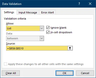
We now have a user-friendly drop-down list for the user to select a Region.
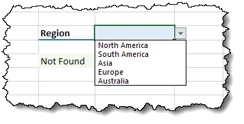
- Select “Australia” from the drop-down list you just created in cell G5.
Let’s step back for a moment and dig a bit deeper into the thought process of the formula.
- Select cell F7 and place yourself in edit mode. Highlight the portion of the formula that represents the include argument (B6:B20=G5).
=FILTER(A6:C20, B6:B20=G5, “Not Found”)- Press the F9 key to display the results of each individual record test against cell G5.

The F9 key is great for debugging formulas. If you are creating complex formulas and need to debug errors or track the flow of logic in a formula, the F9 key is one of the most useful tools in Excel for this purpose.
=FILTER(A6:C20, {FALSE;FALSE; … TRUE;FALSE;TRUE; … TRUE}, “Not Found”)The FALSE responses represent records where the region was not a match to the selected region (G5). The TRUE responses represent records where the region is a match to the selected region (G5).
IMPORTANT: Because the F9 key is a destructive operation, it changes the formula, we need to return our formula to its original state. This is done by clicking the UNDO button or by using the keyboard shortcut CTRL-Z.
- Press CTRL-Z to return the formula to its original state.
EXAMPLE #2 – Filter by Revenue
Starting in cell F13, we wish to display all the records from our data set (cells A5:C20) that have a revenue greater than the value defined in cell G11 (i.e. 45000).
- On the FILTER sheet, select cell G11 and enter “45000” as the comparison value.
- Select cell F13 and enter the following FILTER formula:
=FILTER(A6:C20, C6:C20>G11, “Not Found”)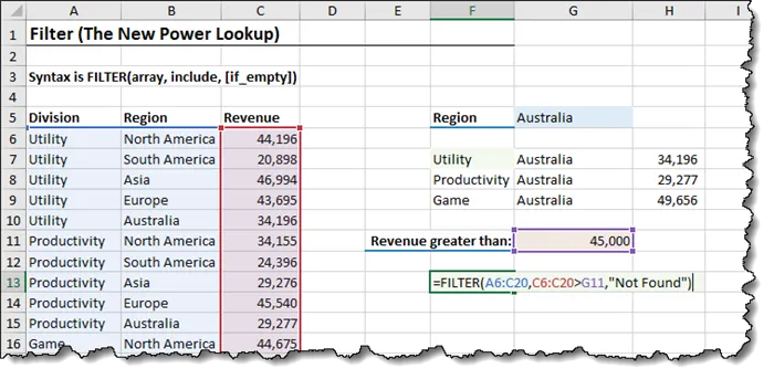
The formula spills and returns all the information from each record where the revenue is greater than the value defined in cell G11 (45000).
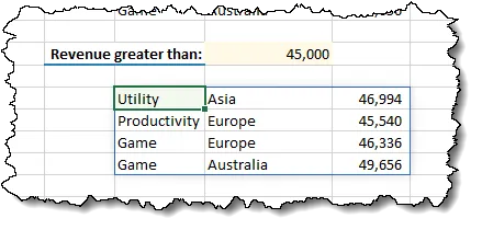
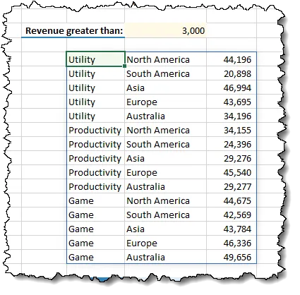
- Test the automatic updating of the formula by changing the revenue in cell G11 from 45000 to 3000. We now see all records within the data set.
Dynamic Array Spill Interference
We need to take into consideration what will happen to an array of spilled answers if the cells being spilled into already contain data.
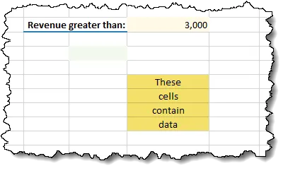
If the spill range contains data from separate activity, the result will be a #SPILL! Error message.
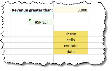
If we click on the #SPILL! error, Excel will highlight the range of cells that were needed to store the result. If the obstructing cells are cleared, the Dynamic Array spill results will appear.
Using Table References with Dynamic Arrays
In the previous examples, we used what is commonly referred to as “plain tables”. This is a table of typed data with no special features added. If we convert the table to a proper Data Table, a variety of new features and additional functionality are bestowed upon the table.
This is typically performed by selecting the table and then clicking Home (tab) à Styles (group) à Format as Table (or by pressing CTRL-T).

When a plain table is converted to a data table, we get a new ribbon of tools for controlling data tables.

For our example, we have a data table that we have named “TableDiv2”.
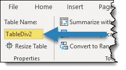
One of the differences when using data tables is the way columns are referenced. Plain tables will display a traditional cell reference when clicked (i.e. =A1), where data tables display what is known as a structured reference (i.e. =TableDiv2[Region] or =[Region]).
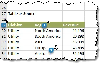
When selecting cells, columns, or entire tables, where you click dictates the way the table is referenced. Data tables have “sweet spots” where clicking can select a cell, a column (field), or the entire table.
Examine the below table and the click locations.
Now let’s see what Excel provides as a reference both in a plain table and a data table.

The best way to determine if a plain table has been converted to a data table is to click on the table and look for the Table Tools Design ribbon.

Just because a table looks “pretty”, doesn’t necessarily mean it was converted; it may have just been artistically customized by hand. The data table functionality may not be available.
EXAMPLE #3 – Filter by Region using Table References
- Copy and paste the Data Validation drop-down list from cell G5 to cell G29.
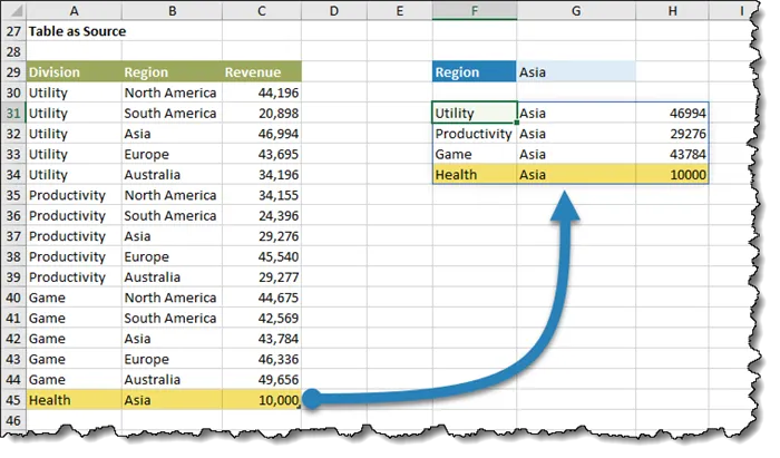
Starting in cell F31, we wish to display all the records from our data set (cells A29:C44) that match the region defined in cell G29 (i.e. “Asia”).
- On the FILTER sheet, select cell G29 and enter “Australia” as the comparison value.
- Select cell F31 and enter the following FILTER formula:
(Tip: When referencing the table in the formula, find the “sweet spot” in the upper-left corner of the table to reveal the thick diagonal arrow. When displayed, a single click will select the entire table regardless of the table’s size. The same can be done when finding the “sweet spot” above the column heading to reveal the thick down arrow. This will select the entire column’s data.)
=FILTER(TableDiv2, TableDiv2[Region]=G29, “Not Found”)
Test the Automatic New Record Detection Feature
One of the advantages of using table references instead of traditional cell references is that when the table expands to incorporate new records, the FILTER function will see the newly inserted records.
Click on the next available cell below the Division column in the data and add a new record for the selected country. Observe how the table has expanded to display the newly added record.
Filtering for Multiple Criteria
Suppose we wish to filter the table for two different criteria: “Game” for the Division and “Asia” for the Region.
- On the FILTER sheet, select cell G37 and enter “Game” as the comparison value for Division.
- Select cell G38 and enter “Asia” as the comparison value for Region.
- Select cell F40 and enter the following FILTER formula:
=FILTER(TableDiv2, (TableDiv2[Division]>G37)*(TableDiv2[Region]>G38), “Not Found”)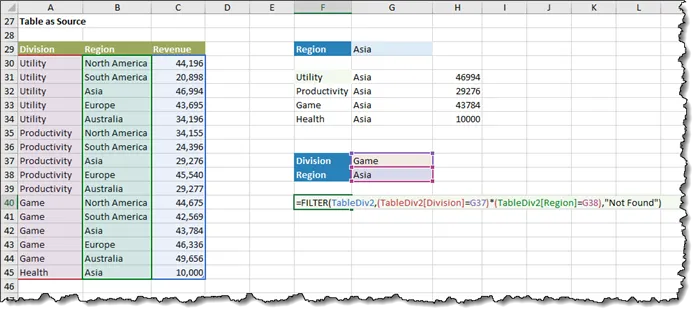
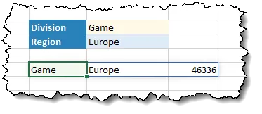
We see all records returned that are “Game” and “Asia”.
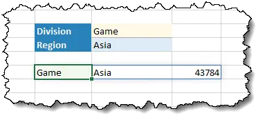
Changing the Division and/or the Region will deliver a different set of responses.
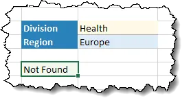
If we were to look for something that does not occur in the data, such as “Health” and “Europe”, we will be presented with a “Not Found” message.
A few points to be made when working with Boolean logic in formulas:
- Because we are potentially returning an array of answers, we can’t use a traditional AND function; we must write the formula using Boolean syntax.
- Each question must be contained within its own set of parentheses.
- The individual comparisons are joined together with an asterisk (*). This creates an AND operation. If we wish to invoke an OR operation, we will use a plus sign (+). We will explore Boolean logic in an upcoming lecture.
Practice Workbook
Feel free to Download the Workbook HERE.

Leila Gharani
I'm a 6x Microsoft MVP with over 15 years of experience implementing and professionals on Management Information Systems of different sizes and nature.
My background is Masters in Economics, Economist, Consultant, Oracle HFM Accounting Systems Expert, SAP BW Project Manager. My passion is teaching, experimenting and sharing. I am also addicted to learning and enjoy taking online courses on a variety of topics.


