#1 – Go To Special (F5)
The Go To Special feature allows you to identify and select items of a specific type. For example, suppose you want to select all cells that contain formulas, or all cells that have had Conditional Formatting applied to them.
Below is the dialog box showing all the selectable item types.
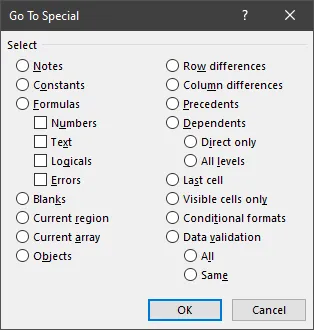
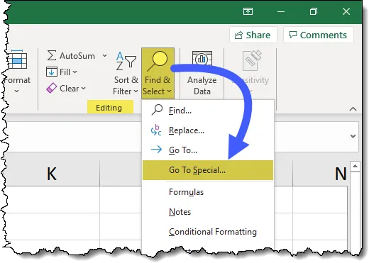
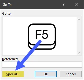
To activate the Go To Special feature you can either click Home (tab) -> Editing (group) -> Find & Select -> Go To Special… or you can press the F5 key or press CTRL-G and click Special… in the lower-left corner of the Go To dialog box.
For some of the more common items discovered by the Go To Special feature, you can invoke their discovery quickly via the “most popular” list.
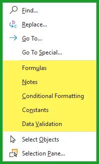
Once a particular type of data is discovered on the sheet (like all cells containing formulas), you could color all the discovered cells, change their font, make them bold, etc.
Featured Course
Fundamentals of Financial Analysis

#2 – Automatic Subtotals (The Subtotal Tool)
The Subtotal tool in Excel allows you to create subtotals for groups of rows without writing any formulas.
The only requirement for the Subtotal tool to perform properly is that the table of data must be sorted by the column where changes in the data are detected.
In other words, if you want to create subtotals of Amounts for each Account, the table must be sorted by the Account column.
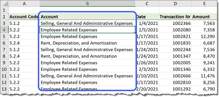
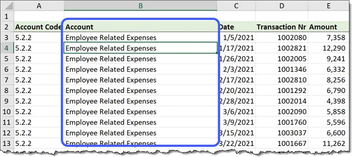
Right-click in the Account column and select Sort -> Sort A to Z.
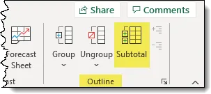
To create the subtotal calculation by the Account groups, select Data (tab) -> Outline (group) -> Subtotal.
This presents a Subtotal dialog box.
From here, we select from the following options:
- Select the column we previously sorted for the “At each change in” option.
- Select the desired aggregation function from the “Use function” dropdown list.
- Select the columns you wish to aggregate when switching between “Accounts”.
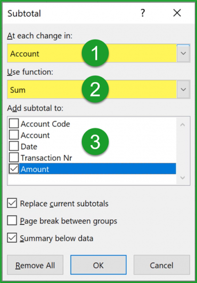
There are other options for controlling the placement of subtotals, page break handling, and deciding on whether to create additional subtotals or replace existing subtotals.
We now have subtotal calculations for each group of “Amounts” for each “Account” along with a total row at the bottom for all “Amounts”.
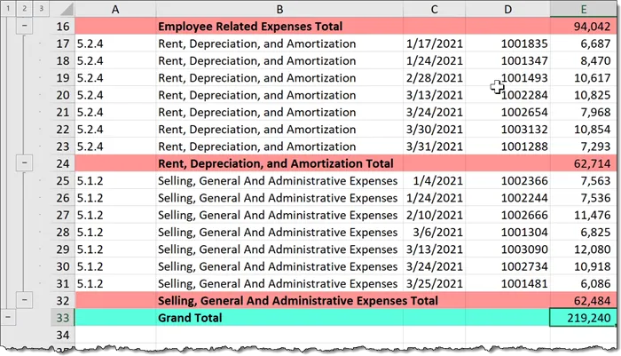
The groupings can be expanded and collapsed to create summary reports by way of the “plus/minus” and “1/2” buttons on the left.
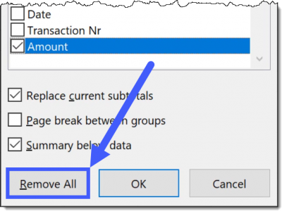
If you need to remove the subtotals, click in the data and select Data (tab) -> Outline (group) -> Subtotal to reopen the Subtotal tool’s dialog box and click “Remove All” at the bottom-left.
Featured Course
Excel Essentials for the Real World

#3 – Number Formatting Shortcuts
It goes without saying that as an accountant you’ll be working with lots of numbers.
Formatting the numbers to provide context and readability is essential, so it’s good to have a quick way to apply this formatting.
If you have a list of dates and you want to apply what is known as the “Short Date” style, you can select the dates and press CTRL-Shift-#.
If you want a date format different from the one supplied by CTRL-Shift-#, you can press CTRL-1 to open the Format Cells dialog box and select from an array of date formats.
To apply a “Currency” style to a list of prices, select the numbers and press CTRL-Shift-4. For a “Comma” style, press CTRL-Shift-1.
#4 – Formula Auditing
When working with many formulas in a workbook, it can become difficult to remember which cells are being used by a formula as well as which cells are being affected by a formula.
If you want to see which cells are being used by a formula, click the cell containing the formula and select Formulas (tab) -> Formula Auditing (group) -> Trace Precedence.

The cells that “feed” the formula are identified by connecting blue arrows.
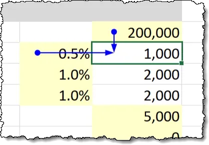
If you want to see which cells are using the data in a cell, click the cell containing the data and select Formulas (tab) -> Formula Auditing (group) -> Trace Dependents.

The cells that use the selected cell’s value are identified by connecting blue arrows.
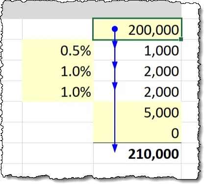
To remove the blue arrows, click Formulas (tab) -> Formula Auditing (group) -> Remove Arrows.

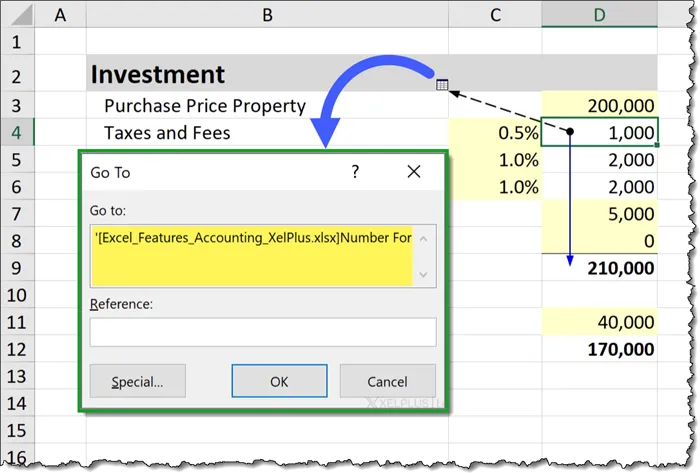
If your precedent or dependent cells are located on a different sheet, a black arrow leading to a table icon is displayed. Double-clicking the black arrow will open the Go To dialog box and display all the sheets/cells where the value is used.
#5 – Conditional Formatting
Conditional Formatting enables Excel to automatically alter the appearance of a cell-based on what is calculated or placed in a cell.
This is a great way to create an alert system to visually notify you of certain events that occur on a sheet, such as coloring a cell green when sales exceed a quota or color a cell red is a safety violation exceed a set value.
You can draw attention to cells based on many different scenarios, such as:
- Values that are greater than or less than a number
- Text that contains specific letters/numbers
- Dates that occur in a set range
- Duplicate or unique values
- Top N or Bottom N values
- All cells that fall within a top/bottom percentile
- All cells that are above or below the average of the set
You can perform a plethora of exotic visuals, such as:
- In-cell bar charts
- Color scales (heatmaps)
- Icon sets
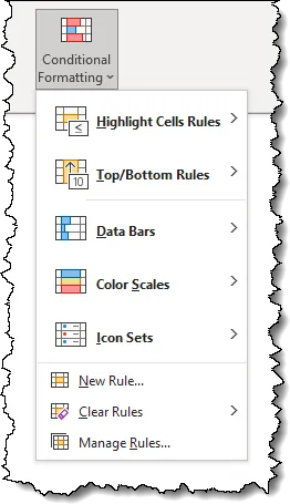
All these features are located on the Home tab under Styles (group) -> Conditional Formatting.
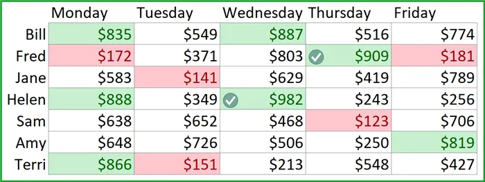
You can layer Conditional Formatting rules to create complex visuals, such as:
- All cells in the Top 20 Percent of sales are shaded green.
- The Lowest 5 sales are shaded red.
- The Top 2 sales get a green checkmark to indicate top performance.
If you need to remove the visual indicators from the cells, you can select Conditional Formatting -> Clear Rules -> Clear Rules from Selected Cells or Clear Rules from Entire Sheet.
#6 – Remove Duplicates
The Remove Duplicates feature will reduce a list of values to only one of each value.
This can be a single-column of values…
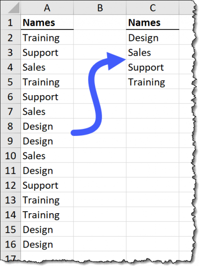
… or a table of values based on multiple criteria.
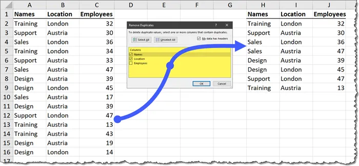
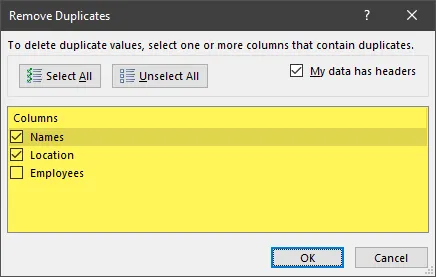
To use the Remove Duplicates feature, click in the list/table of data and select Data (tab) -> Data Tools (group) -> Remove Duplicates.

Select column(s) that you want to be examined for unique items or unique combinations of items.
#7 – Flash Fill
Excel’s Flash Fill (introduced in Excel 2013) is one of the greatest time-saving features when it comes to fixing data.
Flash Fill allows you to “fix” common data format issues like splitting text, merging text, date extraction, text replacement, formatting, and much more.
Flash Fill is located on the Data tab in the Data Tools group and can also be invoked by pressing the CTRL-E keyboard shortcut.

For example, you need to sort a list by the last name, but you were provided a list of names where the first and last names are in the same cell. We need the first names to be in one column and the last names to be in a separate column.
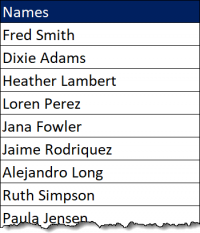
We can split the names by selecting the cell to the right of the first name in the list and typing the first name. After you press Enter, press CTRL-E to generate a list of the remaining first names.
We can now select the first cell to the right of the newly created first names list and type the last name. After you press Enter, press CTRL-E to generate a list of the remaining last names.
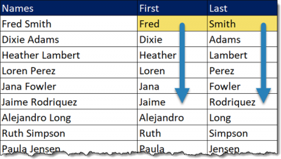
Think of it this way: Type a version of the data the way you WISH it were to appear, then press CTRL-E.
Flash fill can transform data based on a variety of situations, such as:
- Splitting data
- Concatenating data
- Extracting years, months, days, hours, minutes, or seconds
- Replacing data
- Rearranging data
And so much more. Flash Fill is a veritable wonderland of transformation possibilities.
#8 – AutoFilter
The AutoFilter feature provides convenient dropdown buttons at the top of table columns that allow you to sort data as well as filter data based on item selection (via checkboxes) or by a variety of filter criteria.

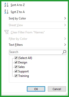
These buttons can be revealed by either selecting Data (tab) -> Sort & Filter (group) -> Filter or by selecting a cell in the data range and pressing CTRL-Shift-L.
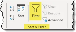
To learn more about AutoFilter and advanced uses of the filter features in Excel, visit the following link to some amazing tutorials.
Excel Filter – Basics to Advanced
#9 – Data Validation
Data Validation is a feature that provides three services to a worksheet:
- Expedites data entry by providing dropdown lists for item selection.
- Limits what a user can type into a cell (ex: prevent text from being entered into a “number only” cell)
- Normalize the data entry by forcing information to be entered the same way (ex: users can enter “football” but not “footballs”, “foot ball”, or “foot balls”)
The links below will showcase many of the uses of Data Validation, but perhaps the single most popular use of Data Validation is for producing dropdown lists.
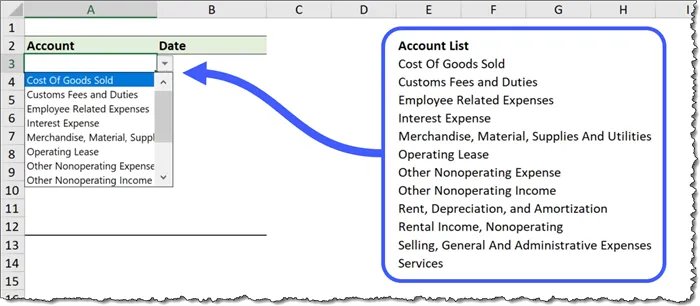
The Data Validation tool is accessible by clicking Data (tab) -> Data Tools (group) -> Data Validation.

For detailed examples using Data Validation, check out the following link to a written post and video.
Excel’s Data Validation Tool
Excel Custom Data Validation
#10 – Pivot Tables
Pivot Tables ranks as one the MOST powerful features in Excel, and the great thing is… they’re really easy to use.
If you can play Computer Solitaire, you have the skills needed to build Pivot Tables.
Pivot Tables allow you to drag-and-drop field names from a list (essentially the labels in your table’s header row) into “zones”. Depending on the zone used, the field’s contents will be either deduplicated and sorted (ex: when using employee names or department names) or aggregated (i.e., totaled, averaged, counted, etc. in the case of sales or profit.)
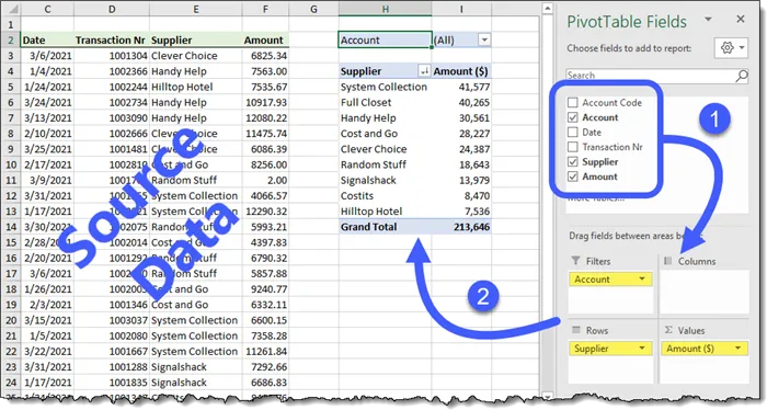
Pivot Tables are one of the best ways to create summary reports without writing a single formula.
The data is reduced, sorted, and aggregated automatically. Color schemes can be applied to the table and the results are easily filtered using dropdown lists or Slicers to answer specific business questions.
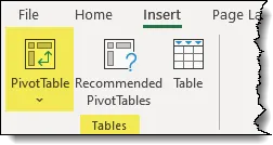
The Pivot Table feature is located on the Insert tab in the Tables group.
One of the best features of Pivot Tables is their ability to update the results when the underlying data changes. Adding, deleting, or modifying data can be pushed to the report with a single click.
To learn how to make and use Pivot Tables in 10 minutes, check out this great written (and video) post showcasing the major features and steps to creating Pivot Tables.
Excel Pivot Tables Explained in 10 Minutes
Leila Gharani
I'm a 6x Microsoft MVP with over 15 years of experience implementing and professionals on Management Information Systems of different sizes and nature.
My background is Masters in Economics, Economist, Consultant, Oracle HFM Accounting Systems Expert, SAP BW Project Manager. My passion is teaching, experimenting and sharing. I am also addicted to learning and enjoy taking online courses on a variety of topics.


