What it is
INDEX and MATCH are “nested” functions – two functions used together.
The first argument of INDEX is to give it an array. This array (range) should include your answer. You then need to specify how many rows to go down and how many columns to move to find the correct value. You cannot move outside the INDEX range.
The syntax of INDEX is:

- The range where the return value resides.
- Number of rows to move down (the row index)
- Number of columns to move to the right (the column Index). This argument is optional. If you only have one column, you can leave the column argument empty, otherwise, you need to specify the number of columns to move over, in the range.
Here is an example of INDEX without MATCH:
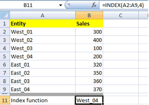
As shown above, INDEX alone is not useful for identifying the number of rows or columns to move. This is where MATCH comes into play. It helps the INDEX function to locate the answer.
The MATCH function was designed to return the position or address of the lookup value to the INDEX function. This is what differentiates MATCH with other functions. It does not return the VALUE in the cell but returns the POSITION of the cell within a specified range.
The MATCH function’s syntax is as follows:

- Like VLOOKUP, Match needs a lookup (target) value. The user can reference a cell or directly type the value into the formula.
- Lookup_array: The “list” (range) where the return values are located.
- Match_type: 0 for an “exact”
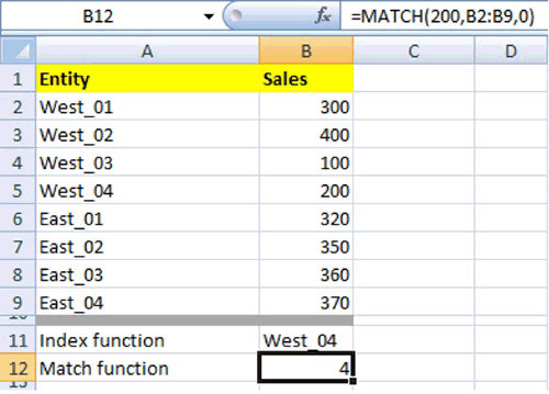
In the below example, the MATCH function returns the value of 4. 200 is 4 rows down from the specified range.
The important point to note on the MATCH function is that it’s a one-way street – you can only have one row or one column selected.
Tip: If your MATCH contains multiple criteria then you need to turn the multiple criteria into a one-way street. You can do this by wrapping the MATCH function inside another INDEX or by converting your formula to an array – CSE – function. To watch this in action, refer to the second part of this guide.
Featured Course
Black Belt Excel Package

Putting it together
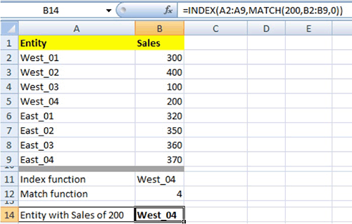
When INDEX and MATCH are used together, the MATCH function finds the look up value’s row / column index and then hands this value off to the INDEX function to get the lookup value. The example below shows how these work in tandem.
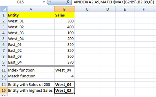
This formula can be further manipulated to find the entity with the highest sales. To do this, simply nest the MAX() function inside the MATCH function to find the location of the highest number.
The VLOOKUP function has to include all the columns in your range even if in-between columns aren’t needed. INDEX and MATCH only requires the return value column which can significantly reduce processing time in larger worksheets.
The easy way to remember the syntax of the INDEX and MATCH is
=INDEX (The range location of my answer, MATCH(The value I’m looking for, The look-up range to find the Value, 0))
Matrix Lookup
Use INDEX MATCH & a second MATCH in cases where you need to look up a value in a matrix. MATCH is used twice: once for the rows and once for the columns. In this example, the return range in the Index function involves multiple columns and the MATCH function instructs the formula to move down a certain number of rows and move over a number of columns across the sheet to retrieve the desired value.
Instead of just selecting a single row or column you need to index the entire table with multiple rows and columns as your array since your value is somewhere inside this matrix.
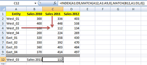
The syntax of the INDEX MATCH MATCH function is:
=INDEX(The full range where your answer can be found in, MATCH(The value I’m looking for in the rows, The range I need to find the Value, 0), MATCH(The value I’m looking for in the columns, The range I need to find the Value, 0))
Building on the INDEX and MATCH Function
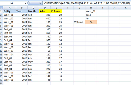
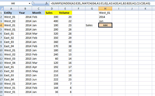
By nesting INDEX and MATCH in other formulas you can create more complex, dynamic calculations. The example below, shows how you can nest INDEX and MATCH in the SUMIFS function. This way you can show the SUM of either the sales column or the volume column depending on whether you select “Volume” or “Sales” in G4. The summing value criteria it uses are West_01 in column A, 2014 in B and Jan in C. Once you change the value in G4 from “Volume” to “Sales”, the results are changed to SUM the values from the sales column. This can be used in dynamic dashboard reports.
INDEX & MATCH is one of my favourite functions because it can be used in many complex situations. A complete understanding of this function is what separates the gurus from the merely capable.
Feel free to Download the Workbook HERE.

Check out Part 2 of this guide, where we go into more advanced uses of INDEX & MATCH.
Leila Gharani
I'm a 6x Microsoft MVP with over 15 years of experience implementing and professionals on Management Information Systems of different sizes and nature.
My background is Masters in Economics, Economist, Consultant, Oracle HFM Accounting Systems Expert, SAP BW Project Manager. My passion is teaching, experimenting and sharing. I am also addicted to learning and enjoy taking online courses on a variety of topics.


