Index Match approach
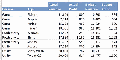
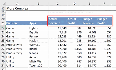
When using the Index Match approach, the first thing you identify is the map or the area that contains the answer. Since this report needs to display the corresponding number from the criteria, the array used is C22:F31. The function at this point is written as:
Cell I22 = INDEX(C22:F31…Had it required to display a value other than the numbers, you will need to include the cells containing those values as well. For example, if you also need to display the Division, the array becomes A22:F31 instead of C22:F31, since A21:A31 contains the Division values.

For the next argument in the INDEX() function, you need to determine how many rows you need to go down. The MATCH() function is used to find at what row number the lookup value is found. Since we want to use the selected App in cell H22 and matching it with cells B22:B31 which contains the Apps, the function now becomes:
Cell I22 = INDEX(C22:F31,MATCH(H22,B22:B31…There are three options for the match type argument:
- 1 = less than
- 0 = exact match
- -1 = greater than
Since we want an exact match, we use 0:
Cell I22 = INDEX(C22:F31,MATCH(H22,B22:B31,0)Find the column that corresponds to both the criteria selected in cells I20 and I21. Another MATCH() function can be used here. Unlike the regular case, your lookup value is derived from two cells. Combine these criteria using the & symbol.

Cell I22 =
INDEX(C22:F31, MATCH(H22,B22:B31,0), MATCH(I20&I21…
The lookup array for this lookup value is found at C20:F21, which has two rows instead of one.
Initially, you would think about using C20:F21 as your lookup array and write the formula as:
Cell I22 =
INDEX(C22:F31, MATCH(H22,B22:B31,0), MATCH(I20&I21,C20:F21,0))
However, instead of displaying the value corresponding to the criteria, it results to an error. This is because MATCH() can only handle a single row or column and cannot handle a combination of rows and columns, such as C20:F21 because it will not know in which direction to move. Had it been a single row such as C20:F20 or C21:F21, it would have worked out fine.
There are multiple ways to resolve this. One way to do it is to revise the table by separating it into two—one containing only the Actual values, and the other containing only the Budget values, and then doing a VLOOKUP to change the source table array depending on the selected criteria. However, it is also possible to resolve this problem without changing the format of the current table. There are three ways to do it.
Method 1: Using helper cells
Since the MATCH() function can only handle single rows and columns, the simplest way to resolve the problem we had earlier is to use helper cells that combine the values in rows 20 and 21 into one row instead of two. This combination becomes the unique identifier of each column.
Cell C19 = C20&C21You will see that C19 now contains ActualRevenue. Drag this formula to the right until cell F19.

Go back to the last MATCH() function that used cells I20 and I21 as the lookup value. Instead of using C20:F21 as the lookup array, you can now use the new helper cells C19:F19.
Cell I22 =
INDEX(C22:F31, MATCH(H22,B22:B31,0), MATCH(I20&I21,C19:F19,0))
This formula displays the value that corresponds to the selected criteria in cells I20, I21 and H22.
Method 2: Using CTRL + SHIFT + ENTER (CSE)
There is another approach that eliminates the use of helper cells. This involves generating an array for the MATCH() function by pressing the keys CTRL + SHIFT + ENTER (CSE).
The MATCH() function is not meant to handle array functions, rather, it looks at things one cell at a time instead of holding things in memory and handle them. Some functions that can handle arrays are:
- INDEX()
- SUMPRODUCT()
- VLOOKUP()
- HLOOKUP()
- AGGREGATE()
However, clicking on CSE on a MATCH() function enables it to handle arrays. Write the same function as above, only instead of using the helper cells, revise the last MATCH() function to combine cells C20:F20 and C21:F21 using the & symbol.
Cell I26 =
INDEX(C22:F31, MATCH(H22,B22:B31,0), MATCH(I20&I21,C20:F20&C21:F21,0))
After pressing ENTER, you will notice that it results to an error because there is no instruction telling the MATCH() function to keep the values in memory. To see the step-by-step calculation of the function resulting to the error:
- Click on cell I26.
- Go to the FORMULAS
- Click on EVALUATE FORMULA.

You will see the function written on the white space. Each click on the EVALUATE button will show you the calculation step-by-step. It first finds the value of cell H22, and finds the row containing that App, followed by finding the values in cells I20 and I21 and combining them. You will notice that the value returned by C20:F20 and C21:F21 are #VALUE! The function notices that you are trying to combine things and it is confused because it does not know how to handle such instances.

Click on CLOSE to exit the window. Go back to cell I26. Click on the function in the formula bar and instead of pressing the ENTER key, click CTRL + SHIFT + ENTER.

Notice that it places { } at the start and end of the function and becomes:
Cell I26 {= INDEX(C22:F31, MATCH(H22,B22:B31,0), MATCH(I20&I21,C20:F20&C21:F21,0))}It now displays the value that corresponds to the three criteria selected.
Click on cell I26 again and go to EVALUATE FORMULA to see how this differs from the previous one. Instead of returning #VALUE! for both C20:F20 and C21:F21, it is now able to find the values in those cells and combine them. The { } gives an instruction to the MATCH() function to keep the values in memory, which makes it easier for it to take C20 and combine it with C21 to give ActualRevenue, D20 with D21 to give ActualProfit, and so on.

It then finds the column number that corresponds to the criteria, “BudgetRevenue”, which is 3. The INDEX() function is now able to find the value using the numbers from the row and column arguments.
This approach is a simple way of writing but it can be confusing for a lot of people. It is only suitable when you are writing the formulas for your own use. Otherwise, if you have other users, it is very likely that those users do not know array functions. They might see the array, click on the formula, inspect it a bit, and press ENTER. Since they press ENTER instead of CSE, the formula will then result to an error again. In such cases, it would be best to avoid this approach.
Method 3: Using two INDEX() functions
The third approach does not require helper cells nor CSE, but replaces the last MATCH() function with an INDIRECT() function.
Start off using the same functions for the most part except for the last MATCH() function:
Cell I29 =
INDEX(C22:F31, MATCH(H22,B22:B31,0), MATCH(I20&I21…
In order to avoid the use of CSE, we need to use a function that can handle arrays. The INDEX() function can be used by putting the entire lookup area inside the INDEX() function. To do this, replace the last MATCH() function in Method 2 with:
INDEX(C20&F20&C21:F21,…It now becomes:
Cell I29 =
INDEX(C22:F31, MATCH(H22,B22:B31,0), MATCH(I20&I21, INDEX(C20:F20&C21:F21…
It is important to comply with the syntax of the INDEX() function. The row_num argument is mandatory. Instead of leaving the formula up until C21:F21, you need to specify a row number. In this case, you want to tell the function to take every single row. There are two ways to do that:
- Use the Excel separator (,) and leave it empty
Cell I29 =
INDEX(C22:F31, MATCH(H22,B22:B31,0), MATCH(I20&I21, INDEX(C20:F20&C21:F21,)…- Use 0 as the row number
Cell I29 =
INDEX(C22:F31, MATCH(H22,B22:B31,0), MATCH(I20&I21, INDEX(C20:F20&C21:F21,0)…
Next, comply with the syntax of the MATCH() function where you need to specify the match type. Again, use 0 for an exact match. The final formula becomes:
Cell I29 =
INDEX(C22:F31, MATCH(H22,B22:B31,0), MATCH(I20&I21, INDEX(C20:F20&C21:F21,0),0))
This gives you the same result as the first two methods. There are other ways to resolve this problem but I find these three to be the simplest ways.
Feel free to Download the Workbook HERE.

Here’s Part 1 of this guide on INDEX & MATCH.
Leila Gharani
I'm a 6x Microsoft MVP with over 15 years of experience implementing and professionals on Management Information Systems of different sizes and nature.
My background is Masters in Economics, Economist, Consultant, Oracle HFM Accounting Systems Expert, SAP BW Project Manager. My passion is teaching, experimenting and sharing. I am also addicted to learning and enjoy taking online courses on a variety of topics.


