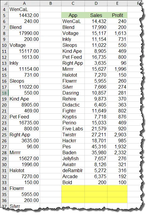
If you have ever tried to take a column of data in Excel like the following…

and transform it into something like this…
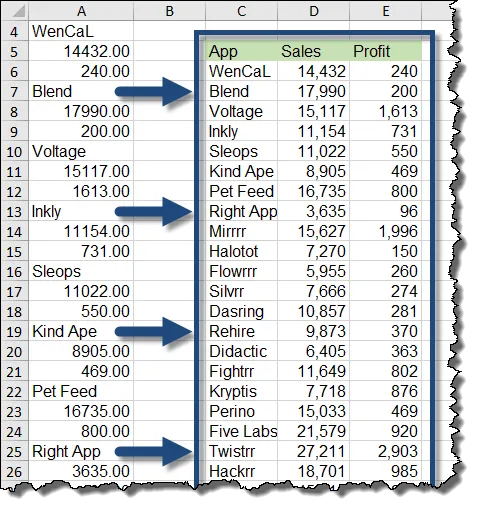
Many different solutions exist for just such a transformation. Some of those solutions include:
- writing a macro using VBA
- developing a Power Query script
- creating an array formula using CTRL-Shift-Enter
- writing advanced formulas using functions like INDEX , COUNTA, ROWS, and COLUMNS
- purchasing third-party add-ins that are programmed for just such a transformation
This post will show you what we consider the “laziest way” to unstack data. But don’t let the word “lazy” turn you away; this may be the FASTEST and easiest way solve the problem.
Step 1: Setup the Headings
In our sample file, we will establish the following headings in cells C5 through E5.

Step 2: Create the Reference Formulas
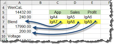
Now create cell references in cells C6 through E6 that create a structure that represents the way you wish the data looked.

Step 3: Implement the “LG” Replacement Trick
Replace the equal signs in cells C6 through E6 with the letters “lg” (these are my initials; feel free to personalize this trick with your own initials.)

Step 4: Create the Pattern References
We need to discover the pattern at which App names appear in the original stack of data. We can see that there is a new App name every third row, just as there is a new Sale value and a new Profit value every third row.
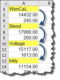
Using our “LG” replacement trick, create a second row of cell references in cells C7 through E7 that are offset by three rows each.
Step 5: Create the Full List of References
Now that we have an established pattern for Excel to work with, highlight all the reference cells (C6:E7). Click and hold the Fill Series handle and drag down. Our original list runs down to row 87. We will produce a list that runs a few references beyond 87 to allow for later expansion of the list.
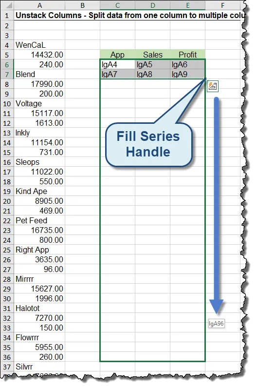
Notice how Excel has recognized the row reference pattern in each column and continued the reference.
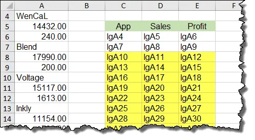
Step 6: Convert the “LG” References to Real Formulas
Select all the cells that contain “LG” references and perform the following Find/Replace operation (Ctrl‑H):
- Find: “lg” (exclude the double-quotes)
- Replace with: = (equal sign)
- Replace All
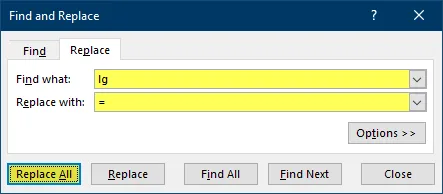
Close the Find and Replace dialog box when complete.
Step 7: Observe Your Beautiful List of Transformed Data
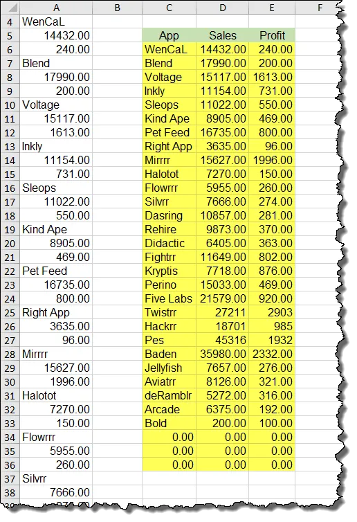
Notice that we have zeroes in the last few rows of the new list. These will automatically update when new items are added to the original list.
If you wish not to see the zeroes, consider applying the following custom number format to the list.
Activate the Format Cells dialog box (CTRL-1) -> Number (tab) -> Custom (category) -> Type (field) and enter the following:
#,##0;-#,##0;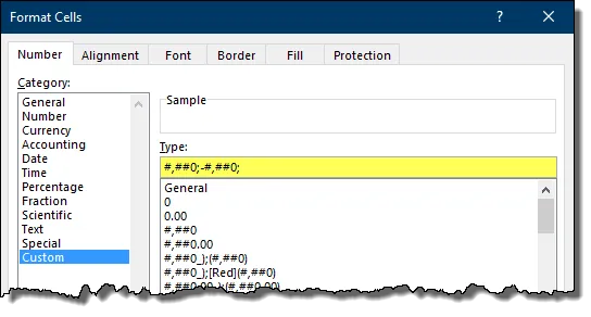
Custom number formats define how positive numbers, negative numbers, zeroes, and text appear. By defining a format for the positive and negative numbers, but omitting the formatting codes for zeroes, Excel will not be able to display a zero value in one of these customized cells.
Featured Course
Black Belt Excel Package

Bonus Step: Adding Additional Data
Because we included additional rows of cell references, if we add a new entry to the bottom of our original stacked list in Column A…

…the newly added data automatically appears at the bottom of our transposed stack of data.

Formula Alternative
If you would rather create a formula, so as not to rely on the “lazy” method, the following formula will produce the desired result:
=INDEX($A$4:$A$87,ROWS($H$6:H6)+(COUNTA($H$5:$J$5)-1)*(ROWS($H$6:H6)-1)+COLUMNS($H$5:H5)-1)Let’s break this formula down.
$A$4:$A$87 is the original list of items in column A.
ROWS($H$6:H6) will count the rows in the defined range. The range expands by locking the first reference and leaving the second reference relative. When the formula is repeated in the descending rows, the row count will increment (1, then 2, then 3, etc…).
COUNTA($H$5:$J$5) will return the number of non-empty cells in the range H5:J5; in this case, 3.
COLUMNS($H$5:H5) will count the columns in the defined range. The range expands by locking the first reference and leaving the second reference relative. When the formula is repeated in the adjacent columns, the column count will increment (1, then 2, then 3).
Using the first instance of the formula in cell H6 to retrieve the first App, the initial evaluations appear as follows:
=INDEX($A$4:$A$87,1+(3-1)*(1-1)+1-1)Which reduces to…
=INDEX($A$4:$A$87,1+(2)*(0)+0)Further reducing to…
=INDEX($A$4:$A$87,1)This will return the item in the first cell of the list; in this case, cell A4 (the app named “WenCal”).
If we look at this for the formula on the same row but for the Sales, we see the following logic:
=INDEX($A$4:$A$87,1+(3-1)*(1-1)+2-1)Which reduces to…
=INDEX($A$4:$A$87,1+(2)*(0)+1)Further reducing to…
=INDEX($A$4:$A$87,2)This will return the item in the second cell of the list; in this case, cell A5 (the sale value 14432).
The formula requires a fair amount of analysis, but to summarize…
ROWS($H$6:H6)+(COUNTA($H$5:$J$5)-1)*(ROWS($H$6:H6) will calculate the location of the next app in the original list.
COLUMNS($H$5:H5)-1 will add 0, 1, or 2 to the previous calculation. This offsets the position to allow for the return of the associated sale or profit value.
Using the Evaluate Formula tool located on the Formulas tab, Formula Auditing group will aid greatly in dissecting the logic in a step-by-step fashion.

Additional Resources
Additional functions that can aid in the transformation of data can be found in the following videos:
Practice Workbook
Feel free to Download the Workbook HERE.

Leila Gharani
I'm a 6x Microsoft MVP with over 15 years of experience implementing and professionals on Management Information Systems of different sizes and nature.
My background is Masters in Economics, Economist, Consultant, Oracle HFM Accounting Systems Expert, SAP BW Project Manager. My passion is teaching, experimenting and sharing. I am also addicted to learning and enjoy taking online courses on a variety of topics.


