Let’s look at an example where we’re trying to determine how much we can invest in a monthly retirement account to achieve a particular return over a set number of years.
The following are the arguments we’ll use in our analysis:
- -$200 – this is how much money we’ll invest in the retirement account each month.
- 20 – this is the number of years till we reach retirement age
- 4% – this is the annual interest rate
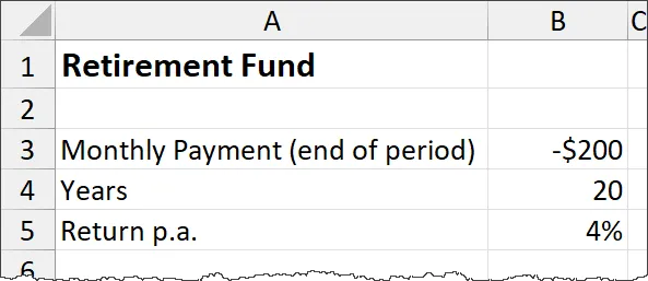
To calculate the amount of money accrued at the end of the 20 years, we can use Excel’s Future Value function (FV).
The FV function calculates the future value of an investment based on a constant interest rate. You can use FV with either periodic, constant payments, or a single lump sum payment.
The syntax for the FV function is as follows:
FV( rate, nper, pmt, [pv], [type] )- rate – (required) The interest rate per period.
- nper – (required) The total number of payment periods in an annuity.
- pmt – (required) The payment made each period; it cannot change over the life of the annuity. Typically, pmt contains principal and interest but no other fees or taxes. If pmt is omitted, you must include the pv
- pv – (optional) The present value, or the lump-sum amount that a series of future payments is worth right now. If pv is omitted, it is assumed to be 0 (zero), and you must include the pmt
- type – (optional) The number 0 (end of the period) or 1 (beginning of the period) indicates when payments are due. If type is omitted, it is assumed to be 0.
For our example, the formula would appear as follows:
=FV(B5/12, B4*12, B3)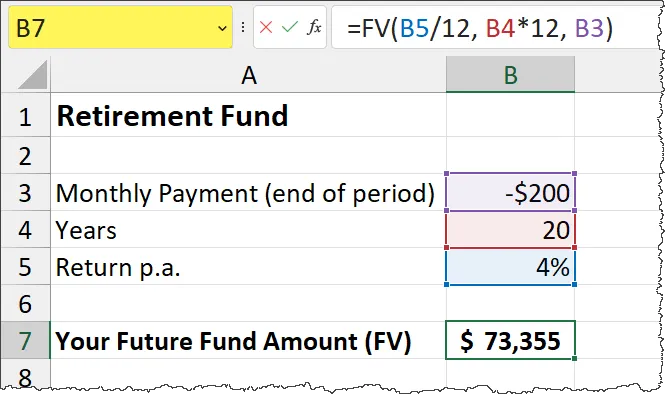
Notice that in the rate argument, we must divide the 4% (cell B5) by 12 because we are paying monthly whereas the rate argument defaults to a yearly period.
The same adjustment must be made to the nper argument for the same reason, multiplying the years (cell B4) by 12.
The monthly payment (cell B3) is a negative value because it is a cash outflow. We’re taking money out of the account.
Featured Course
Excel Essentials for the Real World

Playing the “What If” Game
Suppose we want to see how much money we have at the end of 20 years using different interest rates. We could repeatedly change the “Return p.a.” cell (B7) and try to remember what we saw at each change in the percentage, or…
…we can use the amazing What-If Analysis: Data Table feature.
All we need to do is build our logic prototype as we have here, then use What-If Analysis to build a matrix of calculations for each interest rate we are interested in.
Begin by creating a list of interest rates you wish to calculate against.
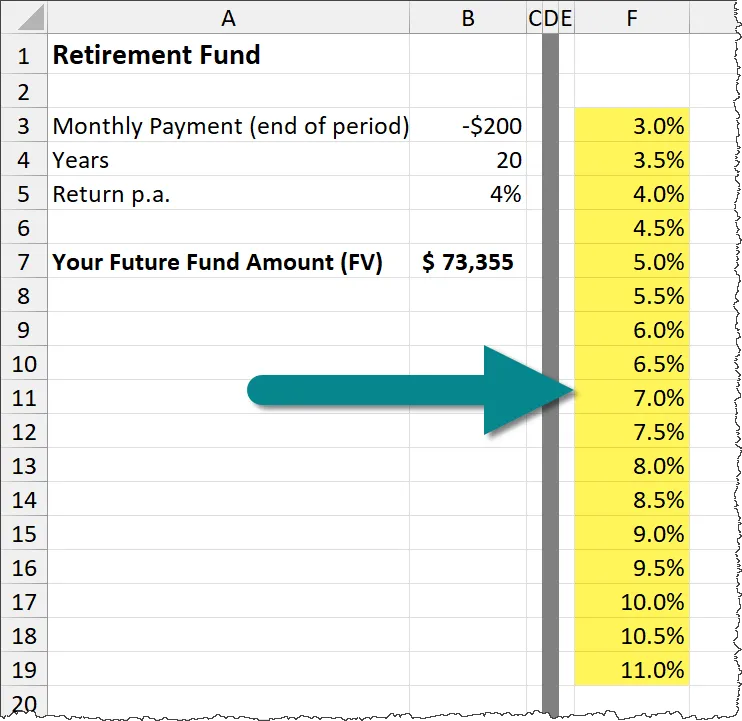
Next, select the cell to the right of the list of interest rates that is 1 row above the first listed rate.

This cell will hold the prototype formula we created earlier in cell B7.
Since we have already created the FV formula, we will simply reference it in this cell.
=B7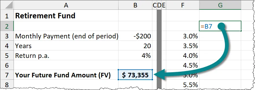
The idea is that we want to repeat the prototype FV formula down this column, swapping out the percentage rate at each row with the rate listed on that same row.
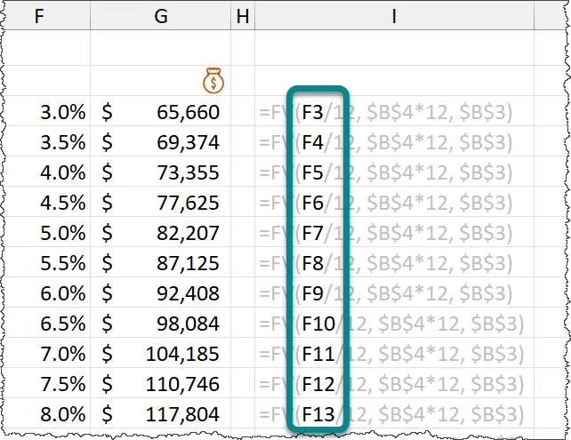
Instead of creating these long, complicated formulas that use a mixture of relative and absolute references (we know how much everyone enjoys those), we can perform the following steps:
- Highlight the range of cells that encompasses the prototype formula, the listed interest rates, and the cells that will display the results (cells F2 through G19).
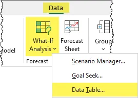
- Select Data (tab) -> Forecast (group) -> What-If Analysis -> Data Table.
In the Data Table dialog box, we must decide whether to use the Row Input Cell or Column Input Cell as the changing range.
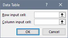
As our interest rates are listed in a column, we will populate the Column Input Cell field.
What we place in that field is a reference to the address of the cell that holds the original percentage rate used by the prototype formula, cell B5.
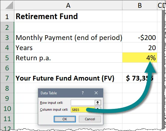
Click OK and we have our table of results for each listed interest rate.
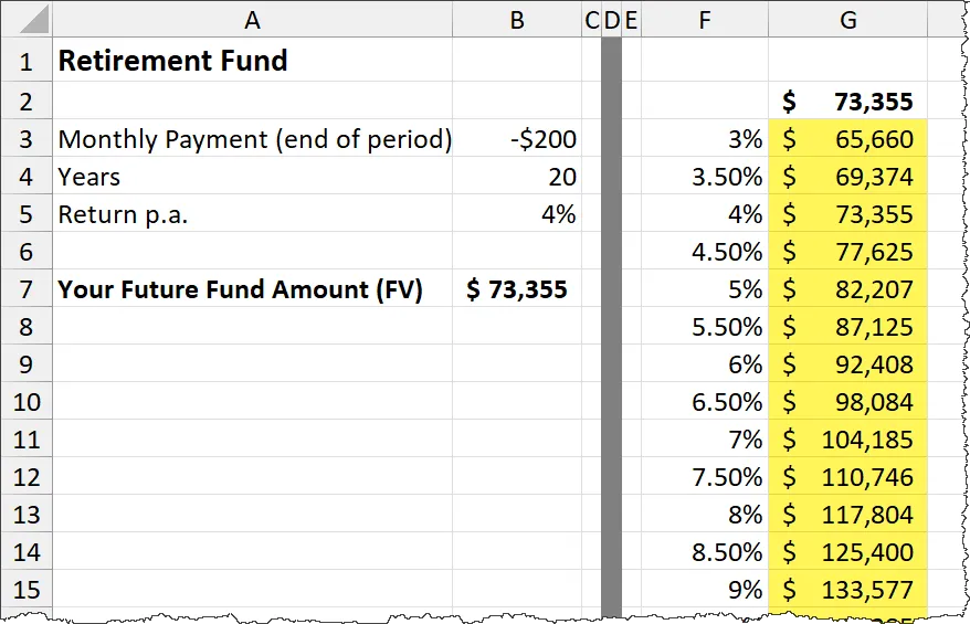
The feature essentially says, “For every reference of cell B5 in the prototype formula, replace it with the value(s) of the cells in the left column of the highlighted range.”
PRO TIP: Customizing the Prototype Formula
One thing that can be a bit confusing for viewers of this table is the repeated result of the prototype formula located at the top of the table.

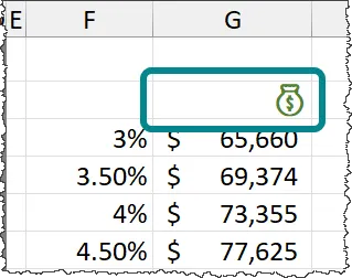
One way to camouflage this formula is to display it as an icon. Perform the following steps:
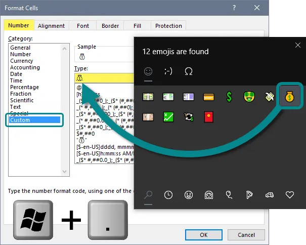
- Select the cell that holds the prototype formula (cell G2).
- Press CTRL-1 to open the Number Formatting
- Select the Custom category (left) and erase everything displayed in the Type:
- Press Windows-Period to open the Emoji library.
- Select an emoji, perhaps something like a bag of money, and press OK.
- Consider changing the font color of the cell to make it more interesting.
Featured Course
Fundamentals of Financial Analysis

Working With Multiple Arguments
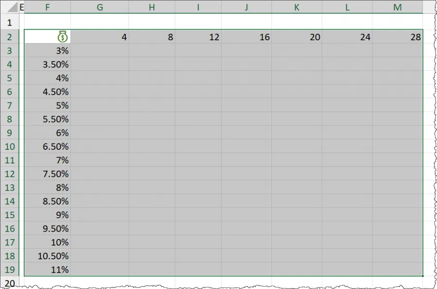
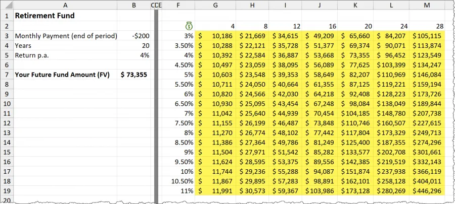
Let’s take this example to a higher level. Suppose we want to show all combinations of the listed percentages against a list of years.
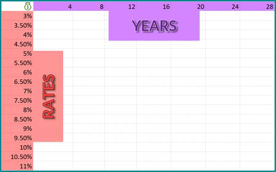
- Move the prototype formula to the cell directly above the first listed interest rate (in this example, cell F2).
- Create a list of years that will reside across the top of the results matrix (in this example, cells G2 through M2).
- Select all cells that contain the prototype formula, interest rates, years, and result cells (F2 through M19).
- Select Data (tab) -> Forecast (group) -> What-If Analysis -> Data Table.
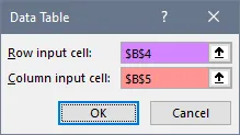
In the Data Table dialog box, the Column Input Cell is the same as before (cell B5), and the Row Input Cell is set to cell B4 (this is the cell reference in the prototype formula that will be changed with each iteration through the top row of listed years.)
Beware of Performance Issues
If you are using the What-If Analysis feature on tables with hundreds of columns and/or thousands of rows, you may encounter a slowdown in performance. This is because the entire data table must be recalculated each time an element in the table is changed.
If you are making several changes, you can hold off on updating the table until all the changes have been made. To do this, we need to adjust the way Excel responds to sheet modifications.
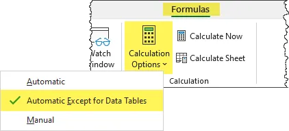
Select Formulas (tab) -> Calculation (group) -> Calculation Options and change this from Automatic to Automatic Except for Data Tables.

Once you have made the needed changes to the table, you can manually update the calculations by pressing the F9 key.
Conclusion
The What-If Analysis: Data Table feature isn’t exactly the most intuitive feature in Excel’s arsenal. It takes a few uses to get the hang of it. But once you’ve used it a few times, it’s actually not that bad, and it can be one of the most useful skills that will easily impress those around you.
Practice Workbook
Feel free to Download the Workbook HERE.

Leila Gharani
I'm a 6x Microsoft MVP with over 15 years of experience implementing and professionals on Management Information Systems of different sizes and nature.
My background is Masters in Economics, Economist, Consultant, Oracle HFM Accounting Systems Expert, SAP BW Project Manager. My passion is teaching, experimenting and sharing. I am also addicted to learning and enjoy taking online courses on a variety of topics.


