Using the RAND Function
The RAND function returns an evenly distributed random real number greater than or equal to 0 and less than 1. As the RAND function is dynamic, a new random real number is returned every time the worksheet is calculated or when you press the F9 key.
The syntax for the RAND function is as follows:
=RAND()NOTE: The RAND function has no arguments, but you are still required to type the parentheses to maintain formula structure.

ANOTHER NOTE: If you are SUPER into random number generation, the RAND function uses the Mersenne Twister algorithm to generate random numbers.
If you want, the result can be formatted as a percentage using the Percent Style.

Fixed Random Numbers
Any change in the workbook (or pressing the F9 key) will force the function to recalculate, generating a new random number.
If you want to preserve the RAND function’s result(s), select the result(s) and perform a COPY / PASTE SPECIAL -> PASTE VALUES operation.
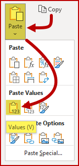
This replaces the formulas in the cell with hard-coded versions of the formula results.
Featured Course
Excel Essentials for the Real World

Using the RANDBETWEEN Function
The RANDBETWEEN function generates a random whole number between two defined values.
This is great when you want to restrict the range of random numbers between a low and high value.
The syntax for the RANDBETWEEN function is as follows:
=RANDBETWEEN(bottom, top)The function arguments are:
- Bottom (required) The smallest integer RANDBETWEEN will return.
- Top (required) The largest integer RANDBETWEEN will return.
To generate a random number between 1 and 100, enter the following formula.
=RANDBETWEEN(1, 100)
As with the RAND function, any change in the workbook (or pressing the F9 key) will force the RANDBETWEEN function to recalculate, generating a new random number.
PRO TIP: If you want to generate a random DECIMAL number between two values, use the RANDBETWEEN and the RAND functions together in a single formula. For example:
=RANDBETWEEN(1, 100) + RAND()
Using the RANDARRAY Function
The RANDARRAY function is a newer function available to Office 365 subscribers and Excel for the Web.
The RANDARRAY function makes it easier to create multiple rows, columns, or arrays of random numbers.
The syntax for the RANDARRAY function is as follows:
=RANDARRAY([rows], [columns], [min], [max], [whole_number])NOTE: All arguments are optional. If you do not define any arguments, the RANDARRAY function behaves in the same manner as the RAND function.
To generate a set of random numbers that occupy 10 cells in a single column, enter the following:
=RANDARRAY(10, 1)To generate a set of random numbers that occupy 10 cells on a single row, enter the following:
=RANDARRAY(1, 10)To generate a set of random decimal numbers between 0 (zero) and 1 that occupy a 10 row by 5 column array, enter the following:
=RANDARRAY(10, 5)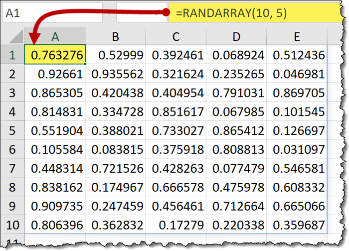
To generate a set of random decimal numbers between 100 and 120 that occupy a 10 row by 5 column array, enter the following:
=RANDARRAY(10, 5 10, 120)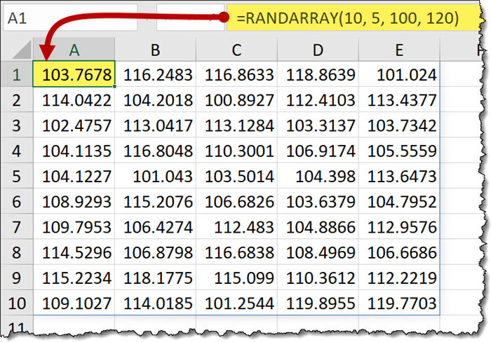
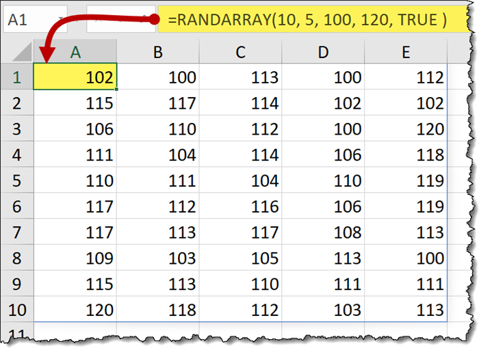
To restrict the values to whole numbers (i.e., integers), place the word “True” in the [whole_number] argument. Using the word “False” in the [whole_number] argument will generate decimal values.
Featured Course
Master NEW Excel Functions in Office 365 & Office 2021

Generate Random Values without Repeats
Encountering repeated values in a list of random values depends on two factors:
- The range by which random numbers are selected (e., the min and max values)
- The number generated values
If you restrict the min/max range to fall between 1 and 10, then generate 100 values, the likelihood of encountering repeats is almost guaranteed.
Generating 10 random values between 1 and 1 million, the odds of encountering repeated values is as likely as winning the lottery three times in a row after discovering the cure for cancer in the letters of your alphabet soup.
If you must use a narrow range of values and require a result with no repeats, place the RANDARRAY function inside a UNIQUE function.
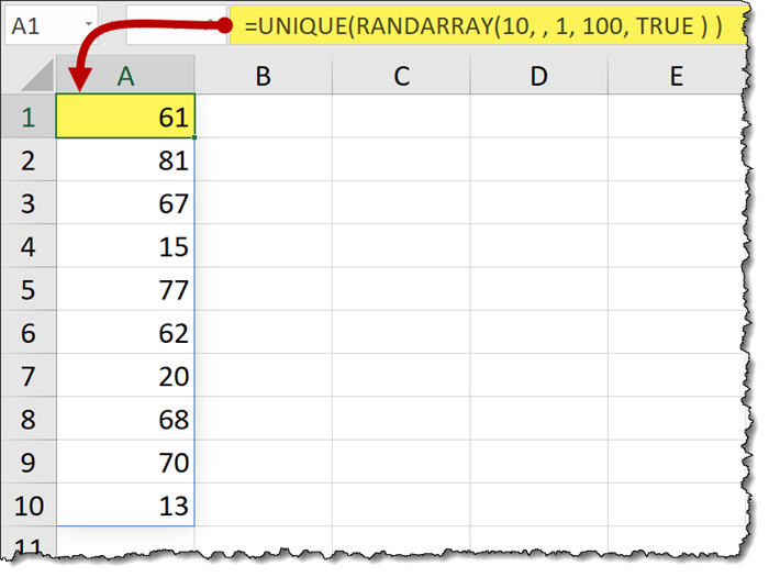
Using this technique, you may encounter (actually, you will more than likely encounter) two issues:
- The result set may shrink and grow with repeated F9 This is because the RANDARRAY function may generate repeated values. If this happens, the UNIQUE function tosses the repeats out. New random, non-repeated values will not take their place.
- A recalculated result array may generate a #SPILL!
SEQUENCE & SORTBY to the Rescue
To work around these issues, you can use the SEQUENCE function with the SORTBY function.
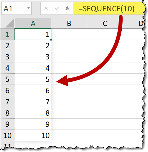
Using the SEQUENCE function, I can generate a list of numbers from 1 to 10 with the following formula.
=SEQUENCE(10)This generates a list of 10 numbers in a single column (10 rows) starting at 1 and incrementing by 1.
To generate a list of 10 even numbers in a single column starting with 2, enter the following:
=SEQUENCE(10, , 2, 2)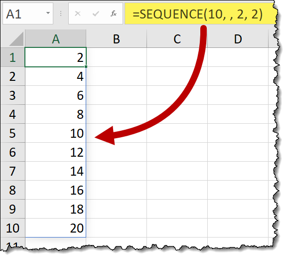
Neither of these examples will ever generate repeats
What if we tool the results of the SEQUENCE function and sorted them in a random order using the SORTBY function?
The SORTBY function can be used to sort an array (ex: our SEQUENCE results) by another array. The second array can be an array of random numbers generated by the RANDARRAY function.
The array of random numbers must be of the same dimension as the SEQUENCE function result.
If we used SEQUENCE to generate even numbers between 2 and 20…
=SEQUENCE(10, , 2, 2)…we nest the above formula in a SORTBY function and define the sort array using the RANDARRAY function.
=SORTBY(SEQUENCE(10, , 2, 2), RANDARRAY(10) )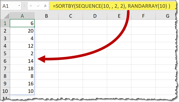
The size is fixed by SEQUENCE and the issue of encountering a #SPILL! error is eliminated.
Generating a List of Random Numbers (Old-School Edition)
If you are using a version of Excel pre-Office 365 and don’t have access to many of these newer functions, here’s a trick that will produce the same results.
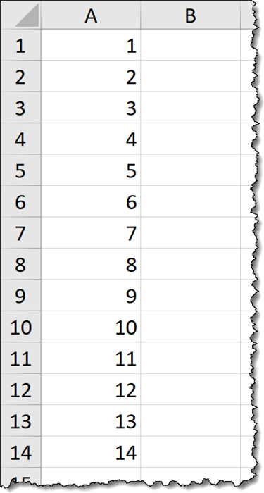
- Create a list of numbers. You can use the Fill Series tool to produce these numbers.
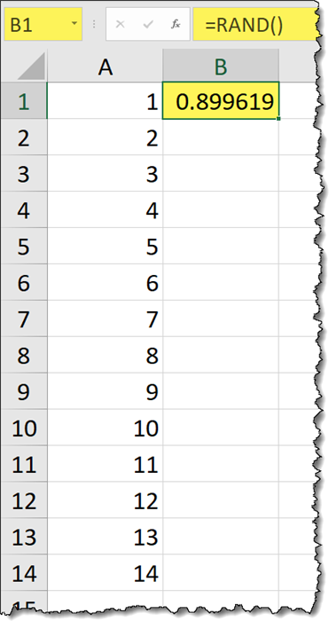
- In the cell directly to the right of the first number in Step 1 list, enter the =RAND()
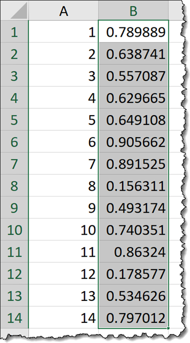
- Fill the newly created RAND() function down the list of original numbers.
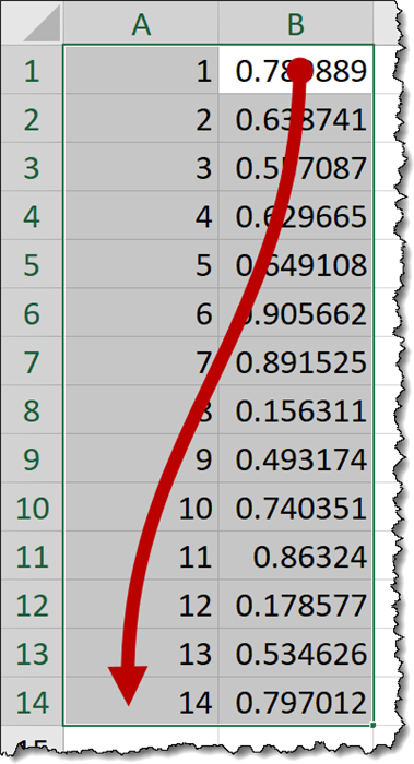
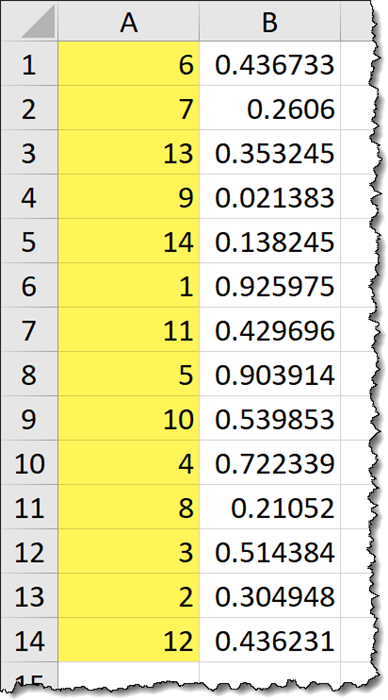
- Highlight the data starting the highlight from the upper-right corner. By starting the highlight from the column of random numbers, you will be telling the next step that the column to sort by is the column you started the highlight with.
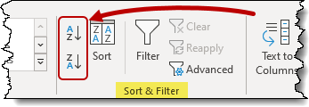
- Click either of the Quick Sort buttons located on the Data It doesn’t matter which one as the “helper column” of random numbers has no inherent order.
Enjoy your randomly sorted list of numbers.
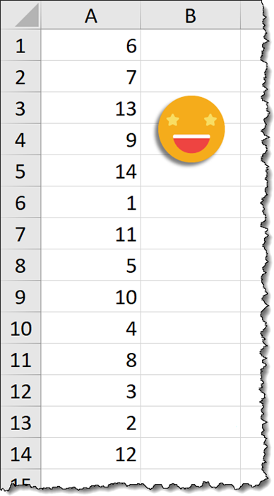
You can feel free to delete the “helper column” of random numbers leaving only the needed values.
Practice Workbook
Feel free to Download the Workbook HERE.

Leila Gharani
I'm a 6x Microsoft MVP with over 15 years of experience implementing and professionals on Management Information Systems of different sizes and nature.
My background is Masters in Economics, Economist, Consultant, Oracle HFM Accounting Systems Expert, SAP BW Project Manager. My passion is teaching, experimenting and sharing. I am also addicted to learning and enjoy taking online courses on a variety of topics.


