This post is an excerpt of my online Google Sheets Comprehensive Masterclass.

This course takes you from a beginner to a Google Sheets expert.
Filter Data by Criteria
We are presented with a dataset…
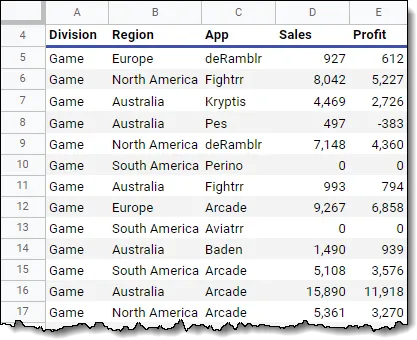
… and we need to perform the following tasks with requirements:
- create a list of Apps, Sales, and Profit
- the list is to be restricted to the selected Region (dropdown selection in cell H6)
- the dropdown list should be generated automatically using Data Validation
- results should be sorted in Ascending order by Proft.
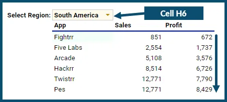
Creating the Dropdown List
To create the dropdown list by which the user will select a Region, perform the following steps:
- Select cell H6
- Click Data -> Data Validation
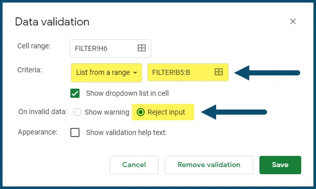
- In the Data Validation dialog box, Set the Criteria to “List from a range” and set the range to B5:B. Set the Data Validation rule to “Reject Input” so the user cannot enter any value not found in the dropdown list.
NOTE: The range reference “B5:B” is not a typographic error. The row reference for the ending cell is purposely omitted. This allows Sheets to “look” for more items when new data is added to the table.
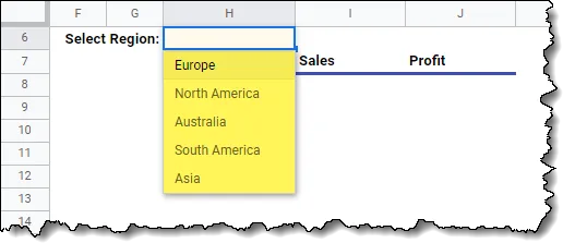
When clicked, cell H6 now presents a dynamically generated list of Regions.
The FILTER Function
The FILTER function is used to produce a table of reduced rows based on an existing table and a set of criteria.
This can be something such as “all records that are from the Country “Austria”, or “all rows with a Sale greater than 100,000”.
The output of the FILTER function includes every row from the referenced table that meets the defined criteria.
The syntax for FILTER is:
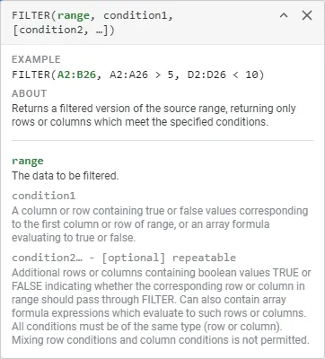
- Range: The Range is the table of data being tested and reduced.
- Condition: The Condition is the logical test by which qualifying rows will be retailed while disqualified rows will be ignored. These tests typically refer to a single column in the table followed by some sort of logical test (ex: “equals”, “greater than”, “less than or equal to”, etc.)
Multiple condition tests can be executed within a single FILTER function.
Filter by Single Criterion (Region)
Using the previously presented dataset, we can write the following formula in cell H8 that takes the selected Region from cell H6 and compares it to the Region column (column B) of the table. If a matching region is discovered, return the data from columns C-D-E of the corresponding row.
=FILTER(C5:E, B5:B = H6)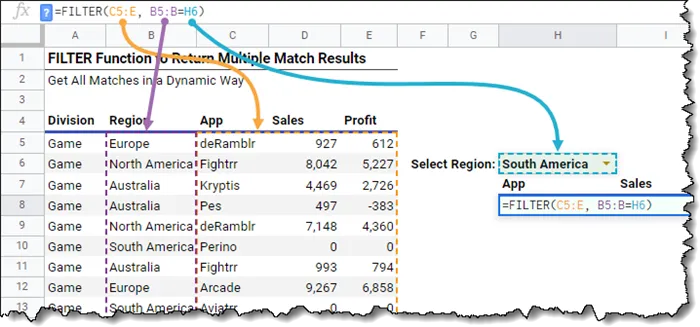
The result is as follows:
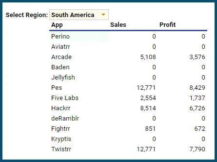
Filter by Multiple Criteria (Region and Sales)
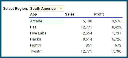
If we wished to refine the result to exclude Apps with zero sales, we can add a second condition to the FILTER function to include only those Apps where Sales is greater than zero.
The updated formula using the second condition would appear as follows:
=FILTER(C5:E, B5:B = H6, D5:D > 0)The result is…
NOTE: If you wished to exclude ONLY zero-valued sales while retaining negative-valued sales, the formula would look like this.
=FILTER(C5:E, B5:B = H6, D5:D <> 0)Sort the Results by Profit
To have the results of the FILTER function sorted from smallest to largest by Profit, we can wrap the FILTER function within a SORT function.
The SORT function allows us to dynamically sort the provided values in either ascending or descending order, and by which columns and in which order.
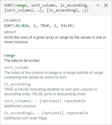
For our purposes, we want to sort the data by Profit (3rd column of the output) in Ascending order. We will use a “3” to indicate the sort should occur on the 3rd column of the output and a “TRUE” to indicate “Ascending” order. Using “FALSE” would invoke a descending sort.
The updated formula would look like so…
=SORT(FILTER(C5:E, B5:B = H6, D5:D > 0), 3, TRUE)
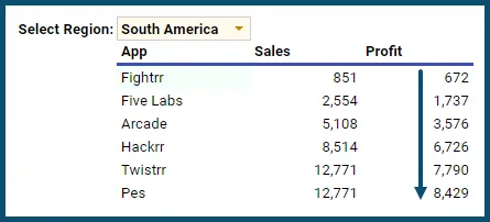
The updated, sorted result is…
Testing the Results
To ensure we have a fully dynamic solution, select different Regions from the dropdown list to see all Apps that were sold to the selected Region that are greater than zero and sorted smallest to largest by Profit.
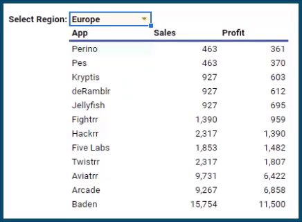
You can also add, delete, or edit records to the data source and see the changes automatically in the FILTER results.
Note to Excel 365 Users
For Excel 365 users who wish to use the Excel equivalent of Google Sheets’ FILTER function, be aware that the argument arrangement is different between Sheets and Excel.

The syntax is mostly identical, but where the FILTER function in Sheets is for additional criteria, Excel’s FILTER function has an option for dealing with filters that return no matching records.
It may appear as if the Excel FILTER function cannot handle more than one criterion, there is a way to have Excel’s FILTER function handle multiple criteria. To see how this is performed, check out this post that shows both in written and video form how to achieve this behavior.
Excel 365 – FILTER Function

Practice Workbook
Feel free to Download the Workbook HERE.
Leila Gharani
I'm a 6x Microsoft MVP with over 15 years of experience implementing and professionals on Management Information Systems of different sizes and nature.
My background is Masters in Economics, Economist, Consultant, Oracle HFM Accounting Systems Expert, SAP BW Project Manager. My passion is teaching, experimenting and sharing. I am also addicted to learning and enjoy taking online courses on a variety of topics.


