In this example, we will use a data set that has Monthly values for each App.
This report enables the user to display a value by selecting an App and a year using dropdown options.
Additionally, we want to highlight this value in the data table.
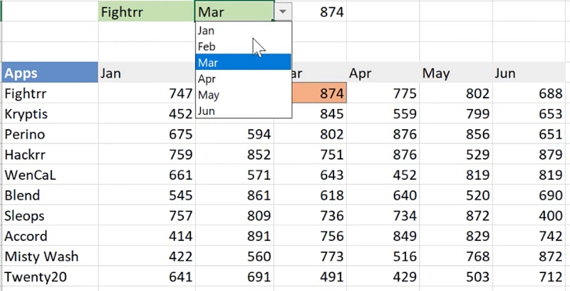
Adding dropdown options for App and Year selections
To create a dropdown option for the Apps, go to the Data tab > Data Validation.

In the Validation criteria, select List.
For the Source, highlight the name of the Apps (cells $A$7:$A$16) and click OK.
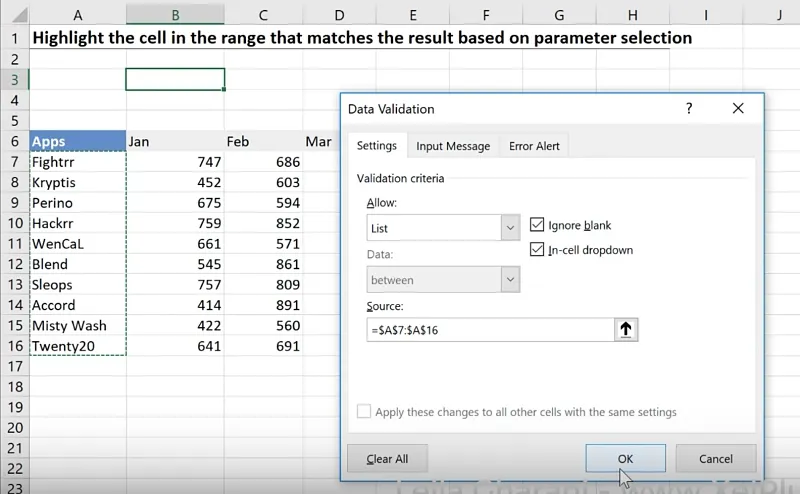
Do the same to have a dropdown selection for the Months, but this time using the cells containing the months (cells $B$6:$G$6) as the Source.
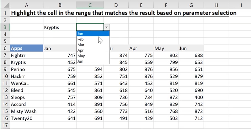
Display the result of the App and Month selection
To find the value corresponding to the App and Month selection, use a formula lookup.
In this example, I am using the Index Match approach (a more detailed walkthrough can be found here).
Cell D3 = INDEX(array,row_num,[column_num])- array – the area where the answer is, B7:G16
- row_num – how many rows down it needs to move. In this case, we use the MATCH() formula to find the name of the App based on the selection. Details about this are found below.
- MATCH(lookup_value,lookup_array,[match_type])
- lookup_value – the value you want to find, in this case the app selected: B3
- lookup_array – where to find this value, A7:A16
- match_type – exact match, 0
- column_num – how many columns to the left it needs to move. Another MATCH() formula will be used to find what column the selected Month is found
- MATCH(lookup_value,lookup_array,[match_type])
- lookup_value – the value you want to find, in this case the month selected: C3
- lookup_array – where to find this value, B6:G6
- match_type – exact match, 0
- MATCH(lookup_value,lookup_array,[match_type])
- MATCH(lookup_value,lookup_array,[match_type])
The final formula is:
Cell D3 = INDEX(B7:B16,MATCH(B3,A7:A16,0),MATCH(C3,B6:C6,0))Highlighting the lookup value in the data set
This lets you visually see where the value is located in the original data set.
Excel’s conditional formatting feature comes in handy here.
A possible approach would be to look up the number result in the data set.
However, this would be a wrong approach since it is possible to have two or more identical numbers in a data set.
This means that if the App Perino is selected for the month of March, this gives a result of 802.
However, 802 also appears under the Fightrr app for the month of May.
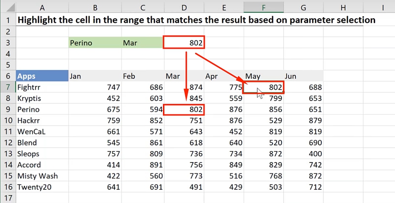
To highlight the correct cell, a check needs to be done for the row and the column based on the selected App and month.
Set up a conditional formatting rule by going to Conditional Formatting > New Rule.
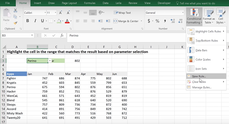
Here you can opt to use a formula to determine which cells to format.
The logic behind is to find what column is equal to the selected month, as well as to find what row is equal to the selected App.
Some challenges in setting up conditional formatting formula rules:
- In the conditional formatting interface, you will not get the Excel help to know which arguments to put in.
- You have to be very careful with fixing the cell references. By default, clicking on a cell gives you a fully fixed cell reference, which might not always be the case. Because you are writing the whole formula from the point of view of the first cell, you would also have to think about how it should apply to the rest of the cells.
To make this easier, type the formulas on the spreadsheet so that you know that it works before transferring it to the conditional formatting rule.
To start off, two conditions need to be met: a cell needs to have the correct corresponding App name and Month. The AND() condition is suitable here.
Cell J7 = AND(B6=C3,A7=B3)Next, determine which cells need to be fixed.
- First argument: Data cell’s month (B6) is equal to the selected month (C3).
- The cell of the selected month is fixed, so the cell reference should be fully fixed as $C$3.
- As for the month of the data cell, it does not change as it moves vertically but changes when it moves horizontally. In this case, only the row reference should be fixed. This gives you B$6.
- Second argument: Data cell’s App name (A7) is equal to the selected month (B3).
- The cell of the selected App name is fixed, so the cell reference should be fully fixed as $B$3.
- The app name of the data cell does not change as the selection moves horizontally. However, it changes when moved vertically. In this case, only the column reference should be fixed. This gives you $A7.
The final formula is:
Cell J7 = AND(B$6=$C$3,$A7=$B$3)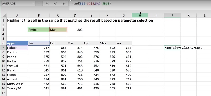
When hitting ENTER, you will notice that if the App Perino and the month of March are selected, the formula results in a “FALSE” because none of the conditions have been fulfilled by cell B7 (Fightrr, January).
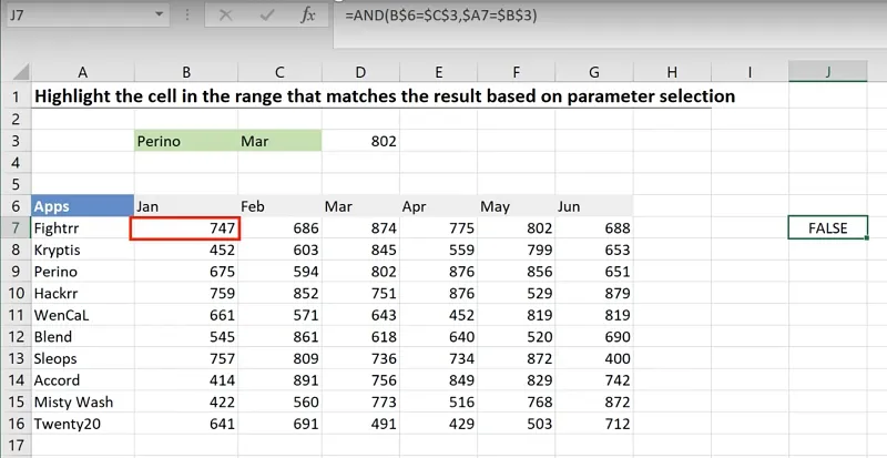
Pull the formula across and all the way down to match the original data set.
This way, you can see if the formula works.
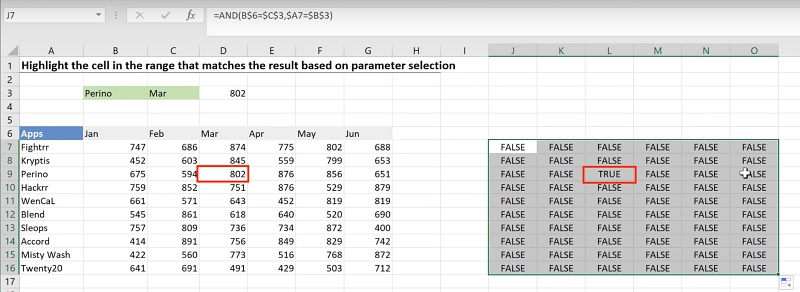
Notice that cell L9 displays as “TRUE” because this corresponds to the App Perino and the month of March.
You can then use the formula in cell J7 in the conditional formatting rule.
Highlight the data set (cells B7:G16) which you want to format conditionally.
As done earlier, go to Conditional Formatting > New Rule.
Select Use a formula to determine which cells for format.
Paste the formula.
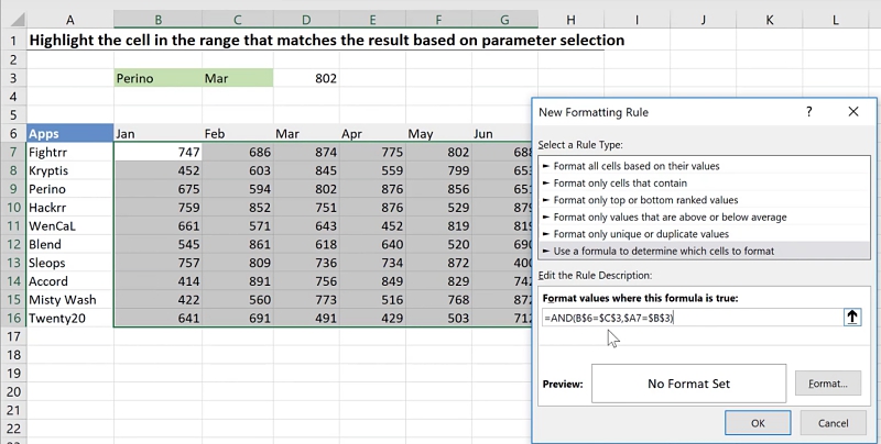
Click Format.
Under the Fill tab, select a color.
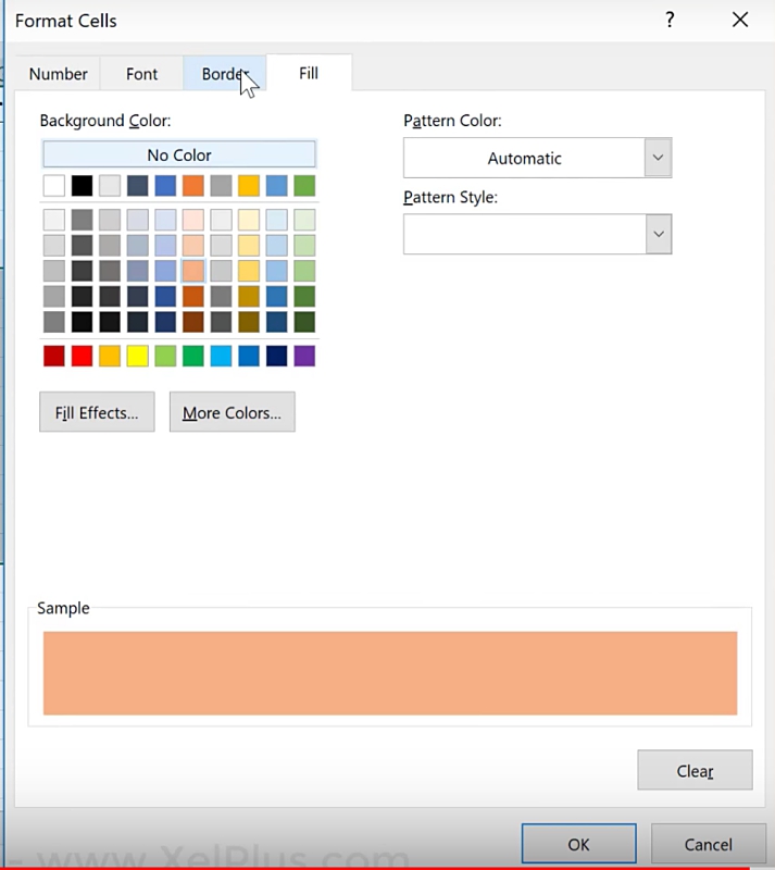
You can also add a border formatting under the Border tab.
Once you have the type of formatting you need, click OK.
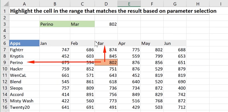
After which, you can then clean up and remove the temporary cells we set up to the right of the original data set.
Feel free to Download the Workbook HERE.

Leila Gharani
I'm a 6x Microsoft MVP with over 15 years of experience implementing and professionals on Management Information Systems of different sizes and nature.
My background is Masters in Economics, Economist, Consultant, Oracle HFM Accounting Systems Expert, SAP BW Project Manager. My passion is teaching, experimenting and sharing. I am also addicted to learning and enjoy taking online courses on a variety of topics.


