What else can it do?
It can also easily solve for the simpler problems that we might face at work.
For example:
- How can we maximize our profit by slightly altering price and costs AND take into account specific constraints for costs and price; such that price cannot go above a certain level and costs cannot go below a certain point. Or:
- How can we distribute the remaining budget dollars among our different projects based on certain constraints?
Solver for Advanced Goal Seek
Goal Seek is restricted to changing only one input variable.
If you have multiple input variables along with some situational constraints as shown below, the Solver function will come in handy.
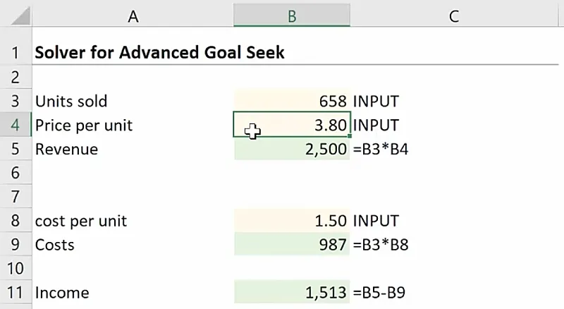
- Units sold: Input variable.
- Price per unit: Input variable.
- Revenue: Calculated field.
Cell B5 = B3*B4- Cost per unit: A fixed number indicating how much each unit costs.
- Costs: Total cost. This is derived by multiplying the number of units by the cost per unit.
Cell B9 = B3*B8- Income: Calculated field. This net income is obtained by subtracting the Cost from the Revenue.
Cell B11 = B5-B9For this scenario, there is a target income of 2,000 and you need to find out how many units need to be sold and the corresponding unit price. It also has the following restrictions:
- Units sold needs to be a whole number
- Price per unit should be between 3 and 4.
Activating the Solver tool
To activate the Solver tool,
- Go to File.
- Click on Options.
- In the Excel Options window, select Add-ins.
- At the bottom, go to Manage add-ins and click Go.
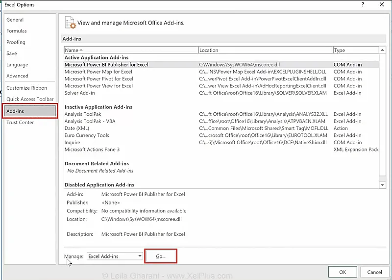
5. Tick on Solver Add-in.
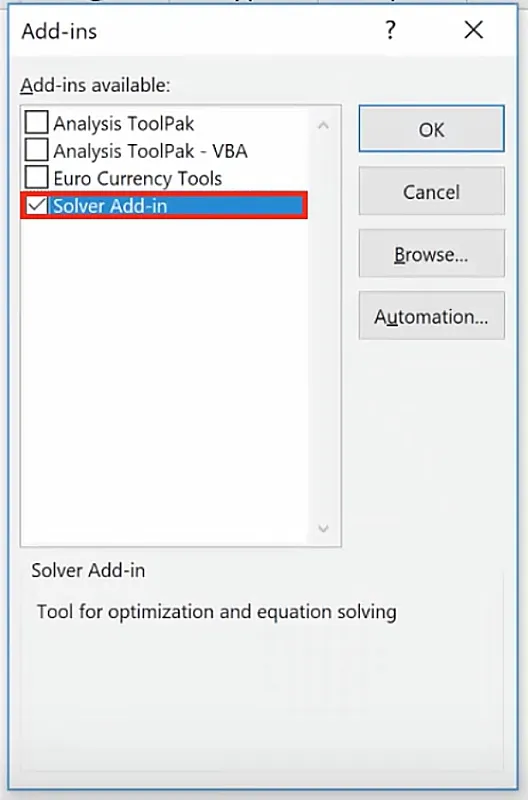
6. Click on OK.
Defining parameters and restraints
The Solver tool is now enabled.
You can find it at the Data tab, under Analyze Section.
To use the Solver tool to find the values we need:
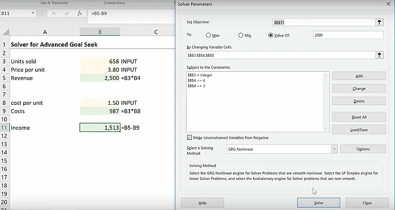
- Set Objective: Cell $B$11, (which is the income ) to a value of 2,000.
- This keeps the income cell fixed to 2,000. Other options allow you to indicate if you are looking for the minimum or maximum value based on the constraints.
- To select variable cells that you want to manipulate, highlight the cells and – when necessary – use a comma as a separator for multiple cells. In this case, use =$B$3:$B$4,$B$8
- To add constraints, click on Add at the right side of the Solver Parameters window. The Add Constraint window will pop up. Select the cell reference you want to add a constraint to. For Units sold parameter, set it to Integer since we want a whole number. Click Add.

- Solving method: GRG Nonlinear.
- Click on Solve. The Solver Results window will pop up, saying that it has found a solution. You will notice that the values of the input cells have changed but the formulas in your calculated cells have been retained. You are given the option to accept the new values by clicking on OK, or reject them by clicking on Cancel.
Types of Solving methods
There are three options for the Solver method:
- GRG Nonlinear – This is the most commonly used method to solve nonlinear problems. This looks for a local optimal solution.
- Simplex LP – This is used to solve linear problems.
- Evolutionary – This is used to solve more complex and non-smooth non-linear problems. It looks for a global optimal solution, which makes it take longer to run compared to GRG Nonlinear.
You can select any of the three options, but by default, the GRG Nonlinear method is used.
Solver for Complex What-if problems with constraints
Consider a scenario where you have to allocate a budget among multiple parameters in the table below:
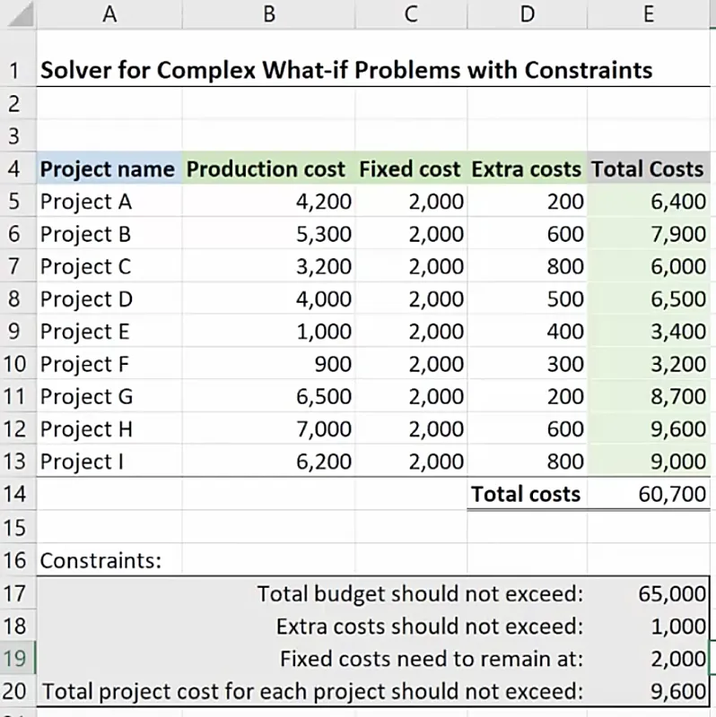
Notice that there are constraints that indicate the following:
- Extra costs should not exceed 1,000
- Fixed costs need to remain at 2,000
- Total project cost for each project should not exceed 9,600
To set it up in the Solver tool, do the following:
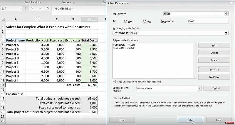
- Set objective: $B$14 to value of: 65000
- Change variable cells:
- Extra costs column: $D$5:$D$13
- Fixed cost is already at 2,000 so you don’t need to change it.
- Production cost column: $B$5:$B$13. We will choose the Production Cost column instead of Total Costs column because the latter is a calculated field with the production cost as the input.
- Constraints
- Extra costs: $D$5:$D$13 <= $E$18
- Total cost: $E$5:$E$13 <= $E$20
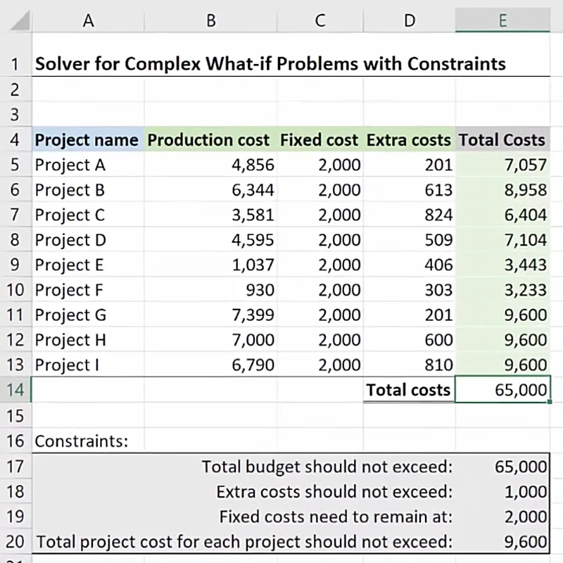
After clicking on Solve, the table will have the new values as follows:
The best way to work with Solver is to experiment.
Start simply and build on it for more complex analysis.
Feel free to Download the Workbook HERE.

Leila Gharani
I'm a 6x Microsoft MVP with over 15 years of experience implementing and professionals on Management Information Systems of different sizes and nature.
My background is Masters in Economics, Economist, Consultant, Oracle HFM Accounting Systems Expert, SAP BW Project Manager. My passion is teaching, experimenting and sharing. I am also addicted to learning and enjoy taking online courses on a variety of topics.


