The syntax of the IF() function is the following:
= IF ( logical_test , [value_if_TRUE] , [value_if_FALSE] )
The first two attributes are obligatory, i.e. without them, the formula doesn’t work, and produces an error message.
- logical _test – a placeholder for the condition we want to test
- value_if_TRUE – an attribute where we need to specify a value (text, or another function) that the IF formula returns when the result of the logical_test is TRUE
The third parameter is Optional, i.e. we can skip it and in such a case, the IF() function returns the default value FALSE.
- value_if_FALSE – an attribute for a value, text or another formula that the IF() function must return when the result of the logical test is FALSE.
In other words, IF() function is used to test the specific conditions and can be described as the statement:
IF something is true, THEN return the first value, ELSE – return then second value.
The simplest IF() function may be written with the first two parameters only.
For example, this formula is absolutely correct:
=IF(C2=1,"Hello!")This formula tests the condition we set (C2=1) and if it is true, the formula returns the text message (“Hello!”).
Otherwise, it returns the default value FALSE.
Interesting Fact!!! You can use another simpler test in Excel for a certain condition. Just place a formula like “=C2>C3” in a cell and press ENTER. If this statement is true, the formula returns the default value – TRUE. Else (i.e. when a value in C2 is NOT larger than a value in C3 cell) the formula will return another default value – FALSE. We use the IF() function in these cases; when we want to trigger some further actions or calculations depending on the results of the logical test.
Typically, the IF() function is used in situations when we need to calculate or flag the results based on certain conditions (for example, smaller than, equal to, greater than and others).
Despite the fact that Excel usually provides multiple choices on how to solve every specific task, the IF() function can play a good role in such cases.
Another simple example of the IF() function:
=IF(C3="Hello!",1, 0)If a value of the C3 cell is the text “Hello!” then this formula returns the one (1) value.
Else (i.e. if this cell contains any other text, number or blank value), the formula returns zero.
The big advantage of the IF() function (like many other Excel functions) is how we can replace all three arguments in this example with whatever we want/need and it still works properly (if we follow the syntax, of course).
For example, let’s replace the one (as a value_if_true) to another formula “C3+C4” and replace zero value (0) to TODAY() function.
Our initial formula becomes:
=IF(C3="Hello!",C2+C3,TODAY())That means – IF a value in C2 cell equals one, THEN do the addition C2+C3.
ELSE (i.e. when C2 doesn’t equal “Hello!”), THEN execute the TODAY() function and return its result.
IF() function is a universal function, i.e. it accepts as an attribute different types of a value, such as numeric value, text, date/time, other functions, named ranges and others).
The IF function can be easily used as a part of other more complex formulas.
Moreover, you can use the so-called nested IF() function and replace the [value_if_false] with another IF() function.
The most common reason to do that is when you need to create a multi-choice comparison like a waterfall.
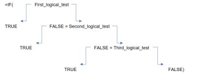
The last value_if_FALSE attribute is a value that we want the formula to return if the result of ALL logical tests in the formula is FALSE.
We know that we need to use a nested IF() (i.e. one IF() inside another IF() statement) when we have a “but” keyword inside the sentence with a logical test.
Take a look at the screenshot below.
In this example, we need to add the text “flag” if a value is greater than 200, BUT if this value is less than 50 we need to return “follow up” text.
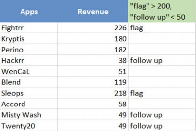
We know that we need to use a nested IF() when there is the “but” keyword in the logical test.
Pro Tip: Be cautious. The more IF iterations we use, the more complex the formula becomes and the more difficult it is to understand. In addition, the complex formulas that contain multiple IF functions along with other Excel functions may slow down the calculation speed, especially if they use large ranges of cells. Also, it’s very easy to make an accidental mistake or typo inside the long and complex formulas, and such errors are difficult to trace properly.
The IF() function is often used with other logical functions such as AND() or OR() functions that we will discuss further.
Let’s look at some practical examples…
TEST CASE №1 Adding the word “Good” if the Revenue is greater than 15000
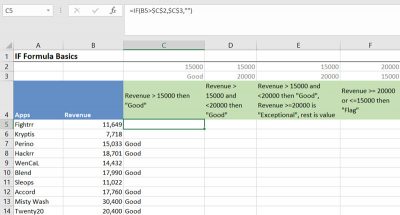
This is a typical use of the IF() function.
Let’s flag all apps if their Revenue is above 15,000.
Step 1. Go to the first cell where we need to insert a formula (cell C5 in this example).
Start the formula with an equal sign (=), add the keyword IF and the opened parentheses to make the formula look like:
=IF(Step 2. The first argument of the IF() function is a logical test.
In this example, we want to flag a value in cell B5 (Revenue) if it is above 15000.
So, let’s continue the formula =IF(B5>15000,
Do not forget to put a comma once this step is ready.
This coma is used by Excel as a delimiter to separate the arguments from each other.
Pro tip: We can either type a numeric value in the logical test or use a cell reference to a cell that contains such a value (C2 cell in our example). The second approach is preferred because it gives us more flexibility in the future. Once we copy/paste the formula to the entire range, all we need to do in this case – if want to change that value – is go to the referral cell and change it there without needing to re-write the formula for all related cells.
NOTE: Keep in mind that if we want to use this approach, we need to fix the cell reference to look like $C$2. This fixed cell address is required for copying the formula to the entire range. Without that, the formula will return the wrong result. We can simply press F4 to fix the cell reference in the formula (make sure that the cursor is located near the appropriate cell address)
The formula becomes:
=IF(B5>$C$2,Step 3. The second argument of IF() function, as we remember, is a value_if_TRUE.
Let’s type the text “Good” as a second attribute in the formula:
=IF(B5>$C$2, "Good",Do not forget to put a comma once this step is ready.
Also, be careful – if you type a text value, you need to put it inside a double quotation mark (“your text”)
Pro tip: We can either type a numeric value in the logical test or use a cell reference to a cell that contains such a value (C3 cell in our example). If in the future we’ll decide to change the “Good” word to something else (“Not Bad”, for example), then all we need to do is go to cell C3 and change that text in the cell without the necessity to re-do the entire formula.
Our formula becomes:
=IF(B5>$C$2,$C$3,NOTE: Don’t forget to fix the cell reference to look like $C$3 address. Press F4 to make an absolute reference. Without that, the formula will return a wrong result.
Step 4. The third argument of the IF() function is value_if_FALSE. We can skip this attribute (in such cases Excel returns the default value – FALSE). However, if we want to do that in a more aesthetic way, let the formula return a blank value. The blank value in Excel is equal to nothing between two quotation marks, like “”. So, the final version of the formula becomes:
=IF(B5>$C$2,$C$3,"")NOTE: Don’t forget to close the brackets and press ENTER.
Step 5. Drag the formula down to the entire range.
Make a quick check manually to ensure that the formula returns the correct result according to our expectations.
TEST CASE №2 Adding the word “Good” if the Revenue is greater than 15000 and less than 20000
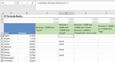
Let’s flag all apps if their Revenue is above 15,000 but under 20,000
Step 1. Go to the first cell where we need to insert a formula (cell D5 in this example).
Start the formula with an equal sign (=), add the keyword IF and the opened parentheses to make the formula look like:
=IF(Step 2. The first argument of the IF() function is a logical test.
In this example, we want to flag a value in cell B5 (Revenue) if it is above 15000 and less than 20,000.
This is a typical situation when we can use the AND() logical function to unite several certain conditions into a single logical test.
AND() function can accept up to 255 conditions as its arguments.
Let’s continue the formula and add the second keyword AND with an opened parenthesis.
Once we’ve done that, we can type both conditions for the logical test inside AND() block and close its second parenthesis.
The formula looks like:
=IF(AND(B5>$D$2,B5<$D$3),NOTE: Don’t forget to fix the cell reference to look like $D$2 and $D$3 address.
Press F4 to make an absolute reference.
Without that, the formula will return a wrong result after we drag it down to the entire range.
NOTE: Don’t forget to use a comma once this step is ready.
This comma is used by Excel as a delimiter to separate the arguments from each other.
Step 2. The second argument of IF() function, as we remember, is a value_if_TRUE.
Let’s add another cell reference as a second attribute in the formula:
=IF(AND(B5>$D$2,B5<$D$3),$C$3,NOTE: Don’t forget to put a comma after the attribute once this step is ready. Be careful. If you type a text value, you need to put it inside a double quotation mark (“your text”)
Step 3. The third argument of the IF() function is a value_if_FALSE.
We can skip this attribute and Excel returns the default value – FALSE.
However, the more aesthetic way to do that is to return nothing (or blank value).
Nothing in Excel is denoted as a double quotation mark without any space:
=IF(AND(B5>$D$2,B5<$D$3),$C$3,"")NOTE: Don’t forget to close the bracket and press ENTER.
Step 4. Drag the formula down to the entire range.
Make a quick check manually to ensure that the formula returns the correct result according to our expectations.
TEST CASE №3 Adding the word “Good” if the Revenue is greater than 15000 and less than 20000. Adding the word “Exceptional” if the Revenue is greater than or equal to 20,000. Otherwise, keeping the values
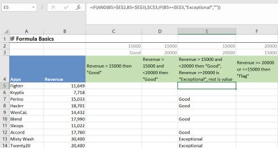
This time we’ll flag all apps as “Good” if their Revenue is above 15,000 and under 20,000.
In addition, we’ll flag them as “Exceptional” if their Revenue is greater than or equal to 20,000
Step 1. Go to the first cell where we need to insert a formula (cell E5 in this example).
Start the formula with an equal sign (=), add the keyword IF and the open parentheses to make the formula look like:
=IF(Step 2. The first argument of the IF() function is a logical test.
The first part of the formula in this example is the same as we wrote in the previous example:
=IF(AND(B5>$E$2,B5<$E$3),$C$3,NOTE: Don’t forget to to put a comma after the attribute once this step is ready.
Step 3. Usually, the third argument of the IF() function is a value_if_FALSE.
However, this time we need to add the second condition when a value in cell B5 is greater than or equal to 20,000.
We can do that if we use nested IF() function.
Let’s add another IF() block as a third parameter now:
=IF(AND(B5>$E$2,B5<$E$3),$C$3,IF(Step 4. Add the second logical test, and the second value_if_TRUE.
In our example, the formula must return the “Exceptional” keyword if the value in cell B5 is greater than or equal to 20,000.
Let’s type this:
=IF(AND(B5>$E$2,B5<$E$3),$C$3,IF(B5>=$E$3,"Exceptional",NOTE: If you type a value as a text, you need to put it inside a double quotation mark (“your text”)
Step 5. We need to write a value that the formula will return if the result of both logical tests is FALSE.
In our example, the formula must return the raw Revenue value in this case.
Let’s place this attribute as the third argument in the second IF() block:
=IF(AND(B5>$E$2,B5<$E$3),$C$3,IF(B5>=$E$3,"Exceptional",B5))NOTE: Don’t forget to close the brackets.
We created two IF blocks, so we need to close two brackets at the end.
Step 6. Drag the formula down to the entire range.
Make a quick check manually to ensure that the formula returns the correct result according to our expectations.
TEST CASE №4 Adding the word “Flag” if the Revenue is greater than or equal to 20,000 OR it is lesser than or equal to 15,000
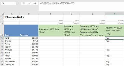
Let’s flag all apps if their Revenue is <= 15,000 or >= 20,000
Step 1. Go to the first cell where we need to insert a formula (cell D5 in this example).
Start the formula with an equal sign (=), add the keyword IF and the open parentheses to make the formula look like:
=IF(Step 2. The first argument of the IF() function is a logical test.
In this example we want to flag a value in cell B5 (Revenue) if it is below or equal to 15000 OR above or equal to 20,000.
This is a situation when we can use OR() logical function that allows the testing of multiple logical conditions and return a true value if ANY of them is true.
Let’s continue the formula and add the second keyword OR with an opened bracket.
Once we’ve done that, we can type both conditions for the logical test inside OR() block and close its second parentheses.
The formula looks like:
=IF(OR(B5>=$F$2,B5=<$F$3),NOTE: Press the F4 button on the keyboard to make an absolute reference.
Step 3. The second argument of the IF() function, as we remember, is a value_if_TRUE.
Let’s add this attribute in the formula:
=IF(AND(B5>$D$2,B5<$D$3),"Flag",NOTE: If you type a text value, you need to put it inside a double quotation mark (“your text”)
Step 4. The third argument of the IF() function is a value_if_FALSE.
Let’s add a double quotation mark without any space to return a blank value:
=IF(AND(B5>$D$2, B5<$D$3),"Flag","")NOTE: Don’t forget to close the bracket and press ENTER.
Step 5. Drag the formula down to the entire range.
Quickly check to ensure that the formula returns the correct result.
TEST CASE №5 Using other formulas inside the logical functions
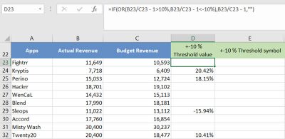
Let’s calculate the difference between Actual Revenue and Budget Revenue and flag those cases when the difference is larger than +/- 10%.
Step 1. The easiest way to start building such a complex formula is to calculate the core value (this is the +/-10% threshold value in our case).
Step 2. Go to the first cell where we need to insert a formula (cell D23 in this example).
Start the formula with an equal sign (=), add the formula to calculate the difference (Actual divided by Budget minus one:
=B23/C23 - 1Step 3. Let’s add the IF() block and the appropriate logical test.
This is a situation when we can use the OR() logical function as we need to flag a value if it is greater than +10% or lower than -10%:
=IF(OR(B23/C23 - 1>10%,B23/C23 - 1<-10%),Step 4. The second argument of the IF() function, as we remember, is a value_if_TRUE.
In this example we need to return the exact deviation, so let’s do that, by simply copying the initial formula.
=IF(OR(B23/C23 - 1>10%,B23/C23 - 1<-10%),B23/C23 - 1,Step 5. The third argument of the IF() function is a value_if_FALSE.
Let’s add a double quotation mark without any space to return a blank value:
=IF(OR(B23/C23 - 1>10%,B23/C23 - 1<-10%),B23/C23 - 1,"")NOTE: Don’t forget to close the bracket and press ENTER.
Step 6. Drag the formula down to the entire range.
Quickly check to ensure that the formula returns the correct result.
TEST CASE №6 Using text symbols as the result of the IF() function
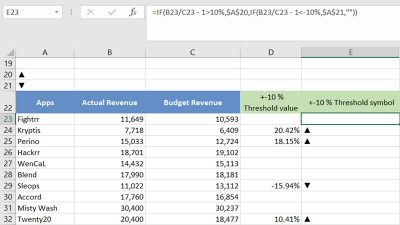
Let’s mark the positive deviation with the up arrow and the negative deviation with the down arrow.
Step 1. We’ll continue the previous example.
Let’s say we want to mark all positive deviations with a symbol that looks like an up arrow and all negative deviations with a symbol that looks like a down arrow.
First of all, a few preparations.
Let’s go to the cells above the test range (A20 and A21 cells in this example).
Feel free to select any other cells if you prefer.
Step 2. Insert the symbols that will indicate all positive and negative deviations.
To do this, we need to go on the INSERT tab on the Excel Ribbon and follow the path: INSERT > Symbol > Arial > Geometric Shapes
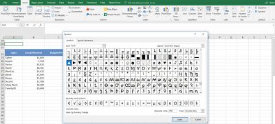
Click Insert once you have selected a shape.
Go to another cell below and insert the second arrow in the same way.
Step 3. Go to the first cell in the range where we want to add these visual indicators.
Replicate the IF() function with the cell references containing the arrows as the value_if_TRUE and value_if_FALSE attributes.
=IF(B23/C23 - 1>10%,$A$20,IF(B23/C23 - 1<-10%,$A$21,""))NOTE: Don’t forget to close the bracket and press ENTER.
Step 4. Drag the formula down to the entire range.
Quickly check that the formula returns the correct result.
Workbook for Download
Feel free to Download the Workbook HERE.

Leila Gharani
I'm a 6x Microsoft MVP with over 15 years of experience implementing and professionals on Management Information Systems of different sizes and nature.
My background is Masters in Economics, Economist, Consultant, Oracle HFM Accounting Systems Expert, SAP BW Project Manager. My passion is teaching, experimenting and sharing. I am also addicted to learning and enjoy taking online courses on a variety of topics.


