Combining Text and Numbers from Separate Cells
We begin with a small table that contains names (text) in column A and amounts (numbers) in column B.
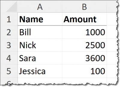
Our goal is to have the name and amount for each row of the table displayed in a single cell (column C).
This needs to be done dynamically so that a change in either the name or amount will trigger an update in the combined version in column C.
This can be accomplished with a CONCATENATE function.
CONCATENATE is a big, fancy word for “join things together”.
Excel has a dedicated CONCATENATE function, but most users will opt to use the simplified version of CONCATENATE… the ampersand (&) symbol.
For example, we begin in cell C2 and write the following formula:
=A2 & B2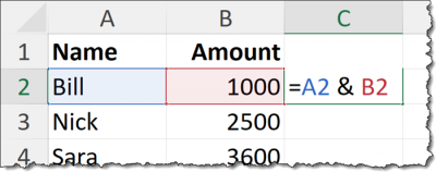
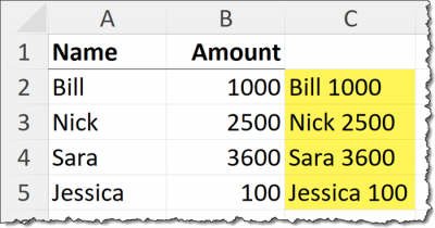
Pressing ENTER to commit the formula results in the following:
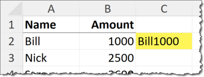
This is the purest form of concatenation; everything is just smashed together. It works, but it’s not visually appealing.
Concatenation is not limited to existing content. We can inject new content into the formula to enhance the results. In our case, we’ll inject a ‘space’ to provide visual padding between the name and the amount.
The ‘space’ needs to be surrounded by double-quotes. Any injected text needs to be surrounded by double-quotes.
=A2 & " " & B2
The updated formula’s result is a bit easier to read.

Think of the ampersand character as the word “and”. “Display the name in cell A2 and a space and the number in cell B2.”
You can place anything you wish between the two double-quotes, like a dash, slash, or any other character.

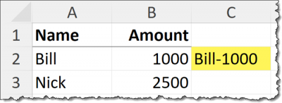
Returning to using a ‘space’, we fill the formula down to the remaining rows to reveal the following:
Featured Course
Excel Essentials for the Real World

Formatting the Numbers in the Result
If we need to represent the numbers in the result as money (we’ll use U.S. Dollars in our example) we can’t just click the dollar sign button on the ribbon. The formatting codes for Currency Style are rendered inert with the presence of the concatenated text.
But not to worry; we have a solution.
We can apply number formatting to the result via the TEXT function.
The Excel TEXT function has the following syntax:
=TEXT(value, format_text)- value – This can be a static value, a reference to a cell that contains a value, or a formula that returns a value.
- format_text – This is the formatting code(s) that determine the way numbers are presented.
For our numbers, we want to display a dollar sign and a comma for every three place values. We also want to show zero if the number is zero.
Our codes for this are:
“$#,##0”
The formatting codes are always placed within a set of double-quotes.
Our formula would be updated as follows:
=A2 & " " & TEXT(B2, "$#,##0")
Committing our new formula to all rows of the tale gives us a much more appealing result.
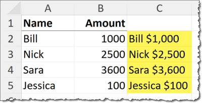
As the values in column B change, the TEXT functions in column C will apply the appropriate number formatting.
For more information on the formatting codes and uses in the TEXT function, visit the following link.
Microsoft Excel’s TEXT Function
PRO TIP:
If you are unsure what formatting codes to use, an easy way to figure it out is to do the following:
- Select a cell with the number you want to format (ex: cell B2) and press F1 to open the number formatting dialog box.
- Select the category (on the left) then the desired formatting (on the right).

- Select the “Custom” category (on the left) to reveal the underlying codes needed to support the selection from Step 2.
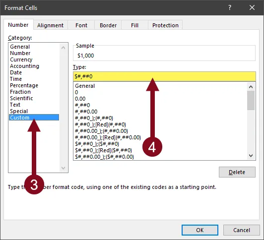
By applying different formatting options and examining the underlying codes, you will likely figure out many of the symbol’s purposes.
Using Aggregation Functions Inside a Formatting Function
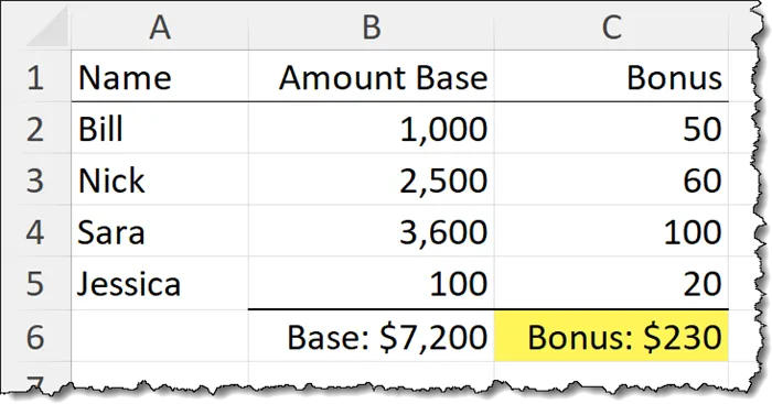
Because the first argument in the TEXT function can be a formula, we can embed an aggregation function, like SUM, into the formula to produce a formatted aggregation.
="Base: " & TEXT(SUM(B2:B5), "$#,##0")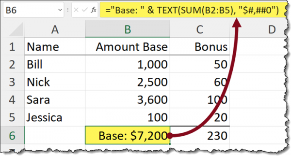
The SUM function provides the aggregation which is then passed off to the TEXT function that applies the formatting codes.
The final touch is to concatenate the text string “Base: ” to the front of the formatted number.
We can write a similar formula for the bonus column.
="Bonus: " & TEXT(SUM(B2:B5), "$#,##0")“What if we want to add the ‘Base” and ‘Bonus’ results?”
If we write a SUM function that attempts to aggregate the results of the previous two formulas, we end up with a less than desirable result.
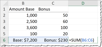
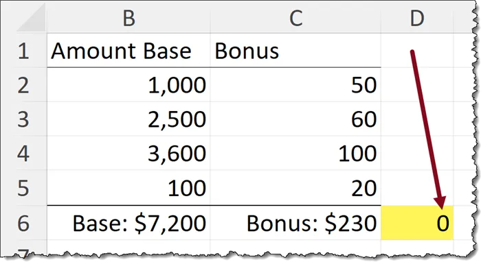
This occurs because we have embedded text in the same cell as the result of the SUM function.
Featured Course
Power Excel Bundle

Separating the Formatting from the Aggregation

We can overcome the previous issue by concatenating the desired text in a Custom Number Format to produce the same result.
This allows you to place a simple aggregation function, like SUM, in a cell without any other modifiers.
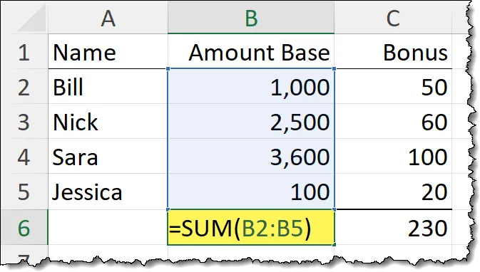
We can then select the cell containing the above formula, press F1 to open the Format Cells dialog box and apply the following custom number format.
"Base: "$#,##0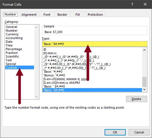
We can apply a similar formatting code sequence to the bonus columns total in cell C6.

"Bonus: "$#,##0Adding the two SUM results now works perfectly.
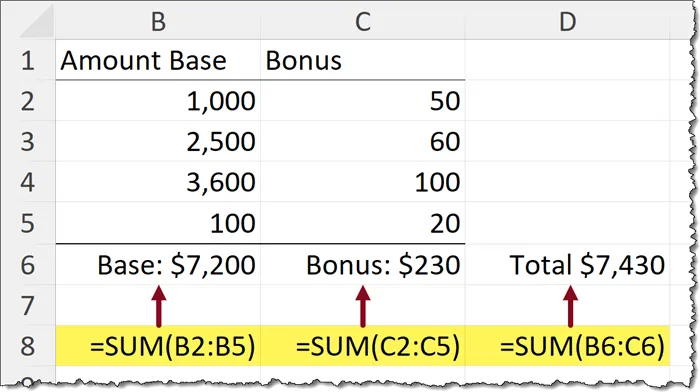
NOTE: I applied the following Custom Number Format to the result to spice it up like the other aggregations.
"Total: "$#,##0Practice Workbook
Feel free to Download the Workbook HERE.

Leila Gharani
I'm a 6x Microsoft MVP with over 15 years of experience implementing and professionals on Management Information Systems of different sizes and nature.
My background is Masters in Economics, Economist, Consultant, Oracle HFM Accounting Systems Expert, SAP BW Project Manager. My passion is teaching, experimenting and sharing. I am also addicted to learning and enjoy taking online courses on a variety of topics.


