Launching the Excel Application
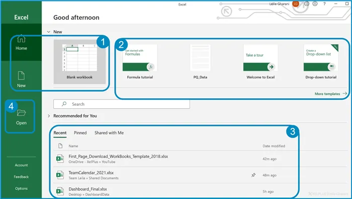
Upon starting the Excel application, you are presented with what is known as the Getting Started page.
This page serves as a branching off point to start or access many different types of Excel files. These include, but are not limited to:
- Starting a brand new blank workbook. This is where you begin when you are starting from zero.
- Starting a brand new workbook based on a template. Templates provide an existing framework with labels, formulas, and sample data. Templates are great if you are in a hurry or lack the needed skills to produce the needed output, such as Pivot Tables or Charts.
- Starting a file from the history list. This is a convenient way to open a file you have been working on in the recent hours or days without having to manually locate the file.
- Open a file not in the history. This is useful for files you may have downloaded from email attachments or recently gained access to via a USB device.
Starting a New, Blank Workbook
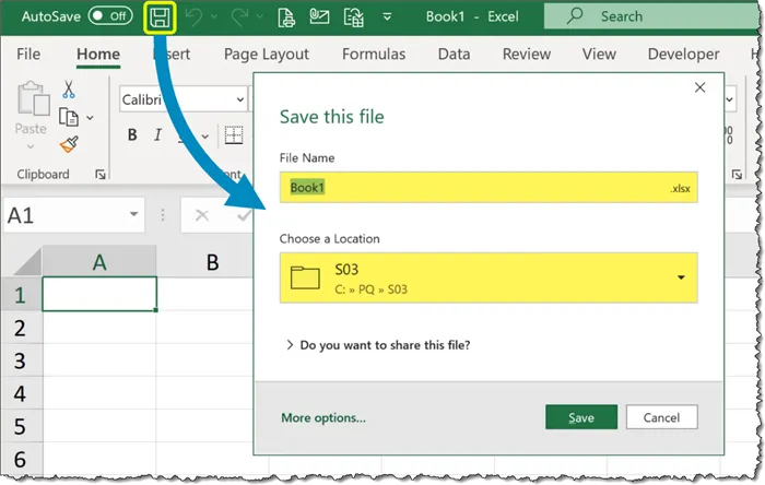
When you begin with a new, blank workbook, the workbook is not saved until you initially save the file.
To save the workbook, click the Save button in the Quick Access Toolbar (upper-left corner), provide a name and location to save the file, and click Save. You can also use the keyboard shortcut CTRL-S.
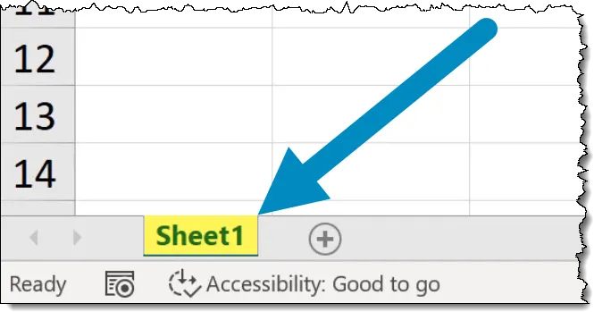
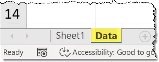
A single Excel file is often referred to as a workbook or spreadsheet. A workbook consists of at least one sheet.
Additional sheets can be added by clicking the “plus” button to the right of the sheet tabs.
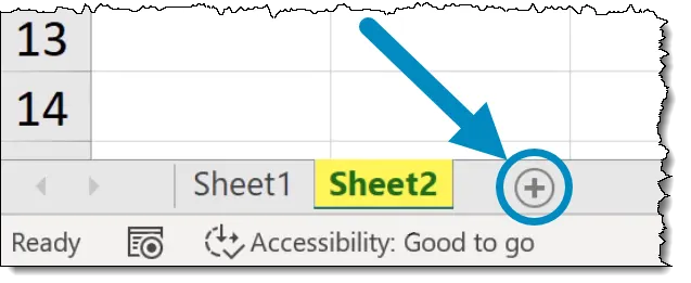
You can rename a sheet by double-clicking on the sheet tab to enable rename mode.
The Layout of the Grid
Each sheet in a workbook is composed of a series of rows and columns. Where these rows and columns interest we have what are called cells.
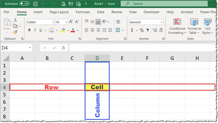
Each sheet has the following dimensions:
- Columns = 16,384
- Rows = 1,048,576
- Cells = 17,179,869,184
This means you can place over 17 billion pieces of unique information on a single sheet.
Entering Data into a Cell
To enter information into a cell, click on the desired cell and start typing. If the cell began as an empty cell, the newly entered data will be displayed. If the cell contains information, that information will be replaced with the newly entered data.
Featured Course
Excel Essentials for the Real World

Cell Addresses
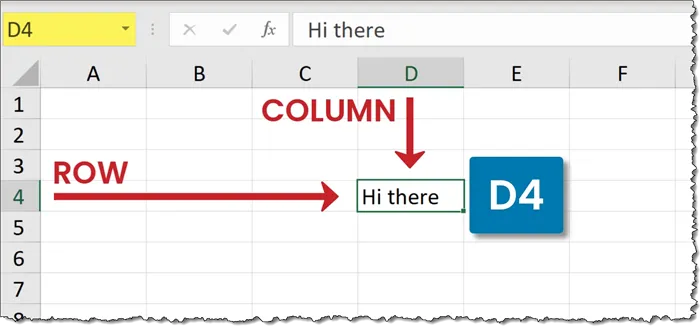
Each of the over 17 billion cells on a sheet has a unique address. The address is a composite of the cell’s column position (a letter) and the cell’s row position (a number).
The Formula Bar
The Formula Bar is where formulas, numbers, or text can be edited after being placed in a cell.
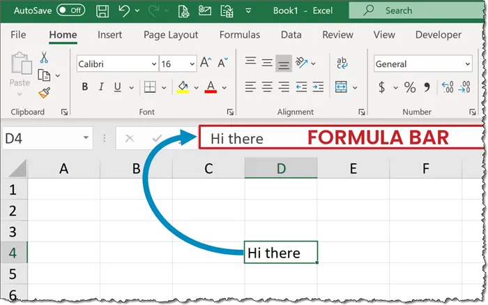
Although you can edit the contents of a cell directly on the grid, this becomes more challenging when working with complex formulas or long passages of text. Performing the edits in the Formula Bar will prove a much easier task.
A cell containing numbers or text will display the same information on the Formula Bar as is displayed in the cell.
A cell that contains a formula will display the formula in the Formula Bar and the formula’s result in the cell.
The Name Box
The Name Box serves several purposes. One purpose is to display the address of the currently selected cell.
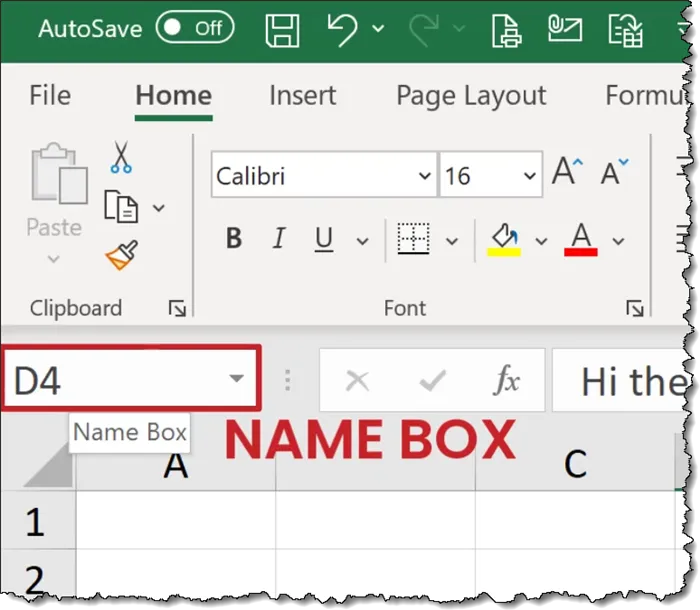
This will make it easier to accurately determine the address of the selected cell, especially if you happen to be zoomed out to a point where reading the row and column headings become difficult.
“Teleporting” to a Cell
When you need to position yourself in a cell that is a considerable distance from your current location, you can type the address of the destination cell into the Name Box and press Enter. This will instantly relocate you to the new cell.
Try the following cell address to see the end of the spreadsheet universe (lower-right corner of the sheet.)
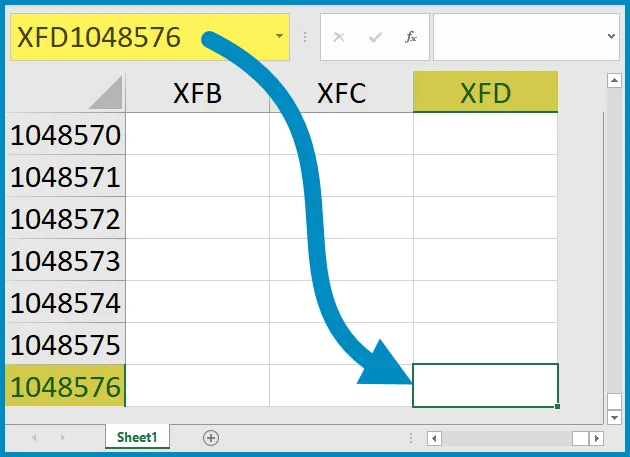
To return to the “beginning” of the sheet (upper-left corner of the sheet) enter the cell address A1 into the Name Box and press Enter. You can also press the CTRL-Home keys to instantly relocate to cell A1.
Selecting Single/Multiple Rows & Columns
To select a row or column, click the applicable row or column header.
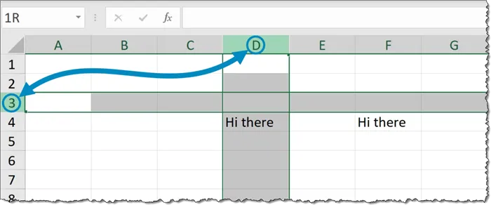
To select multiple rows or columns, click and hold the first row/column, then drag across the adjacent rows/columns until you have selected all the needed locations.
Shortcuts Galore
Excel has more shortcuts than probably anyone knows (at least anyone with a social life.)
One of the best shortcuts for selecting columns is CTRL-Space.
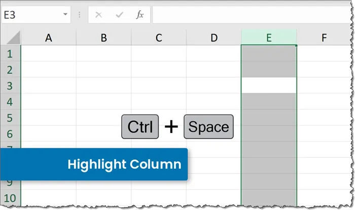
With the column selected, holding the Shift key while repeatedly pressing the left/right arrow keys will select multiple adjacent columns.
NOTE: If you want to see a demonstration of many of the most popular Excel keyboard shortcuts, check out this post and video:
Right-Click Menu
When you right-click a cell, you will receive a menu of options. The options displayed are directly related to the object you have right-clicked on.
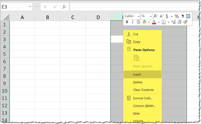
With selected columns or rows, clicking the Insert or Delete options in the right-click menu will either add or remove columns or rows in the same quantity selected.
Coolest Way to Add/Remove Rows & Columns
When you select a row or column, or a series of rows or columns, you can press the CTRL-plus or CTRL-minus keys to quickly add or delete rows or columns.
It is likely to be easier to perform this using the plus/minus keys on the numeric keypad. If you use the plus/minus button located above the letter keys, you will have to add the extra step of using Shift when using the plus key.
Moving to the Extents of the Sheet or Data
You can use the CTRL key along with the up/down/left/right arrow keys to navigate to the extent of the sheet, or if you have existing data, the extent of the data range.
Defining Ranges of Cells
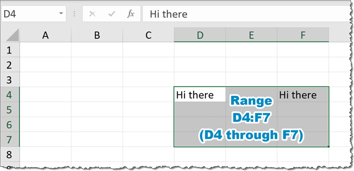
An important term to understand is the word Range. A Range is either a single cell or a group of cells.
When we define a range in a formula, we always refer to the range starting from the upper-left corner of the range to the lower-right corner of the range. We place a colon between the two range addresses to symbolize the word “through”.
Selecting and Moving Cells
When you move your pointer around the grid, you will see a large white plus symbol known as the General Select symbol.
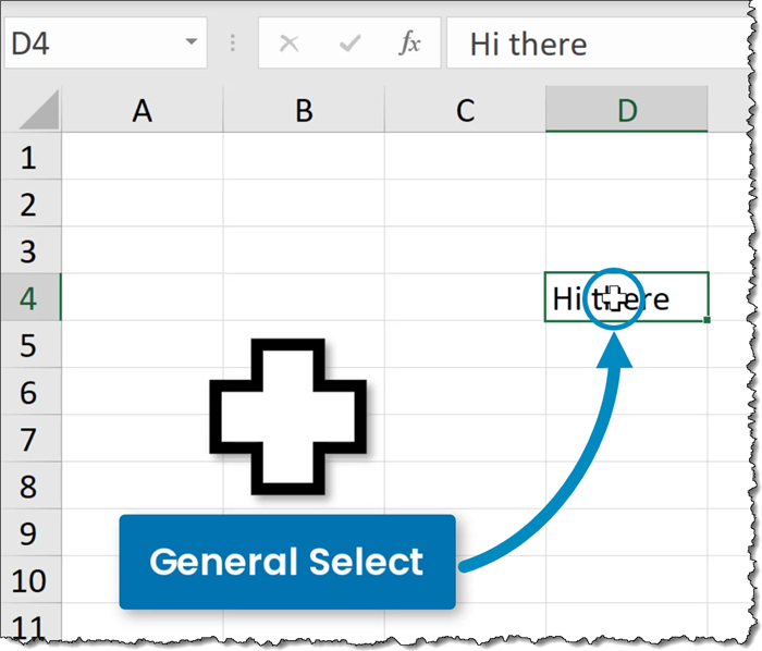
Placing this symbol in the center of a cell and clicking will select the designated cell.
If you place your General Select symbol in the green edge of the selected cell, you will see the large, white plus change to a thinner, black directional arrow known as the Move icon.
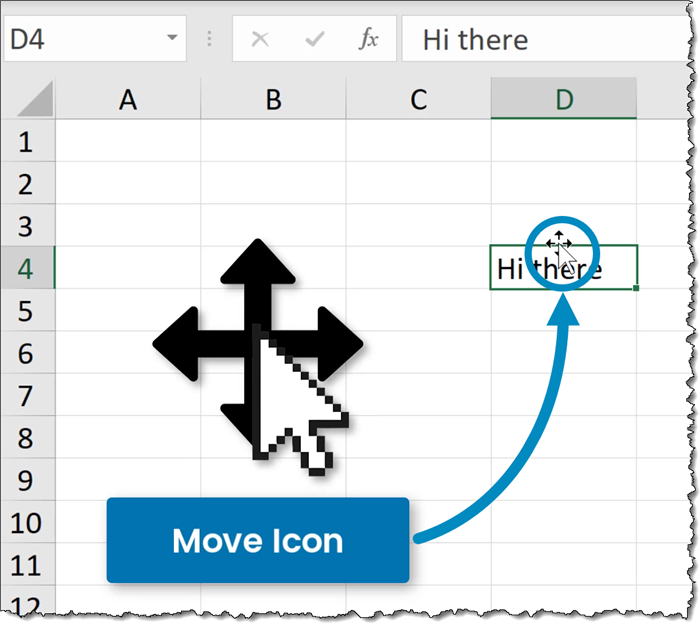
If you click and drag from the green border, you will move the selected cell or range of cells.
If you need to move data between sheets, workbooks, or great distances on the same sheet, you can use the traditional Cut-Paste technique.
The Fill Series Handle
One of the greatest data entry time-savers is the Fill Series handle.
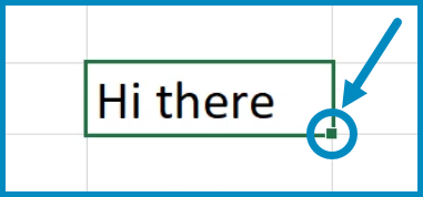
When you place your pointer over this green handle, your large, white plus symbol will change to a thin, black plus symbol.
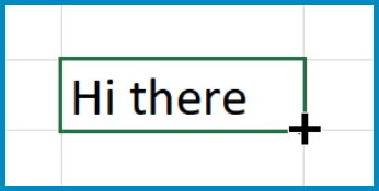
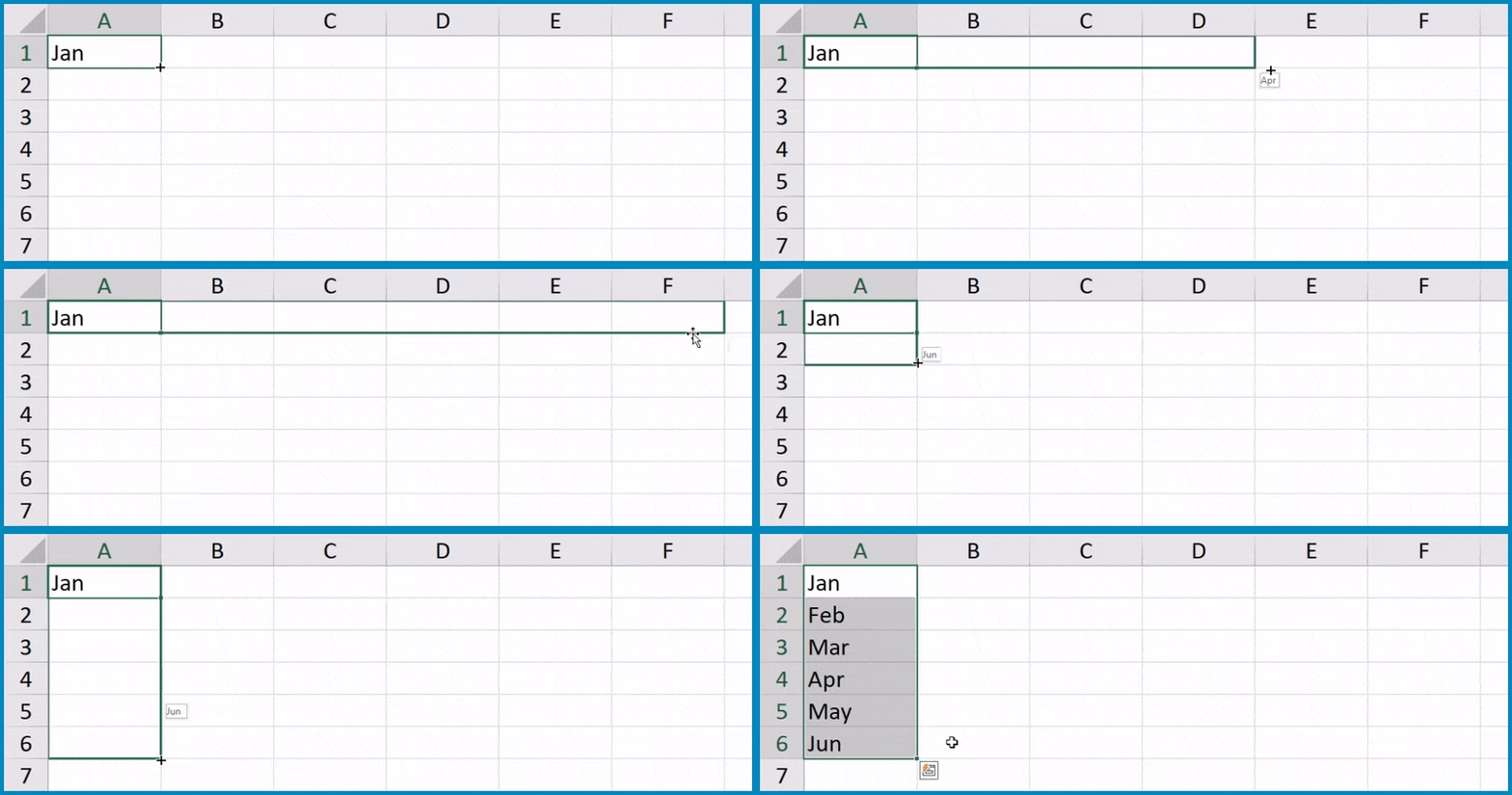
When you see this symbol, click and drag it down or to the right to invoke the Fill Series feature.
Below is a shortlist of things the Fill Series feature will perform:
- Repeat text
- Create lists of months
- Create a list of weekday names
- Create lists of days
- Repeat formulas
- Repeat cell formatting
Resizing Rows and Columns
If you require more width for your columns (typically for text entries), you can hover your pointer over the right column divider (i.e., the divider between columns D & E to resize column D) and click to drag the divider left or right as needed.
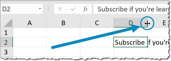
You can perform the same operation on rows by selecting the bottom divider for a specific row and drag up and down as needed.
If you place your pointer over a column or row divider and double-click the mouse, you can invoke an “Auto-Fit” command. This will enlarge or shrink the row/column to the optimal size based on the data contained on that row or column.
Wrapping Text within a Cell
If you don’t want to have an overly wide column to accommodate the contained text, you can activate the Wrap Text feature to have the text automatically apply in-cell carriage returns based on the data and the size of the cell.
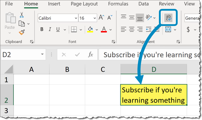
You can remove this feature by selecting the wrapped text cell and clicking the Wrap Text button to toggle the feature to the off state.
Touring the Ribbon
The Tabs and the Ribbon provide access to many of the program’s features.

Clicking the various Tabs will reveal collections of similarly purposed features.
Most of the structural changes made to sheets, like paper size, margin sizes, paper orientation are found on the Page Layout ribbon.

The most used features of the program are located on the Home tab/ribbon.
Learning About Buttons
If you are unsure as to what a particular button will do for you, you can hover your pointer over the button to reveal the “Tell me more” information.
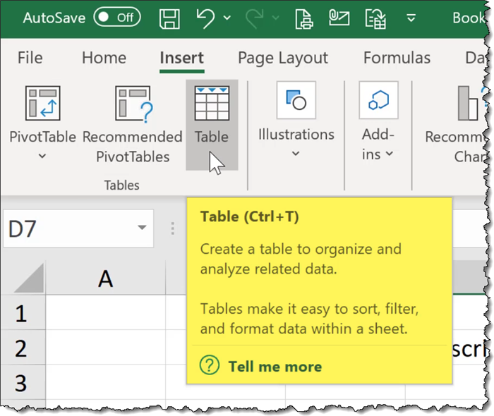
This provides a brief explanation of the button’s purpose, its keyboard shortcut key sequence (if applicable), and a link to open the official Microsoft documentation page for the feature.
Accessing the “Deep Dive” Features
Many of the Ribbon groupings have more features than can be displayed without making the Ribbon overly complicated. For these lesser-used features, you can click the “additional options” button located in the lower-right corner of the button group.

These will open various dialog boxes that contain additional features related to the button group’s overall purpose.
Giving More Space to the Grid
If you want to give more screen space to the grid (and less to the Ribbon), you can either click the “Collapse the Ribbon” button (upper-right corner) or press the CTRL-F1 key combination.

The Ribbon will be hidden leaving only the Tabs visible.

The Ribbon is still accessible by clicking a Tab, but it will automatically hide once it has served its purpose.
NOTE: You can also double-click a Tab to apply or remove this auto-hide behavior of the Ribbon. Many users “discover” this feature accidentally by double-clicking a Tab and thinking they have just lost their Ribbon. Not to worry; double-clicking a Tab will remedy the situation.
Accessing the Backstage
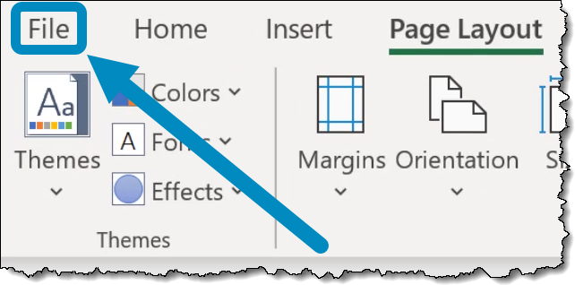
Clicking the File tab will reveal the Backstage.
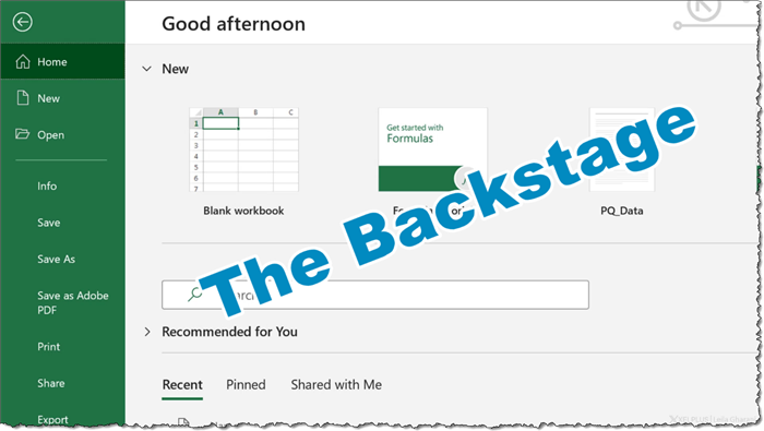
The Backstage is where you go to manipulate the file as an object.
What I mean is you are trying to perform actions such as:
- Save the file
- Open a file
- Close a file
- Print a file
- Email the file
- Convert the file (ex: PDF, or delimited text)
- Protect the file (e., password to open or password to edit)
- Obtain file statistics (ex: size, author, creation date, last saved date, etc.)
Shortcuts for Inputting Values
Getting Out of Edit Mode
When entering data, pressing the Tab key will move the cursor right to the next column, while pressing Enter will move the cursor down to the next row.
If you wish to enter the data without relocating the cursor, press CTRL-Enter.
Getting Into Edit Mode
If you need to edit the contents of a cell, you can select the cell and then press the F2 key. This will enable Edit Mode and place your cursor at the end of the cell’s contents.
Repeating Cell Data
If you have text, numbers, or formulas in a cell, select the cell and adjoining cells to the left or below then press either CTRL-R or CTRL-D to repeat the first cell’s contents to the other selected cells either to the right on the row or downward (below) in the column.
Confining the Data Entry Cells
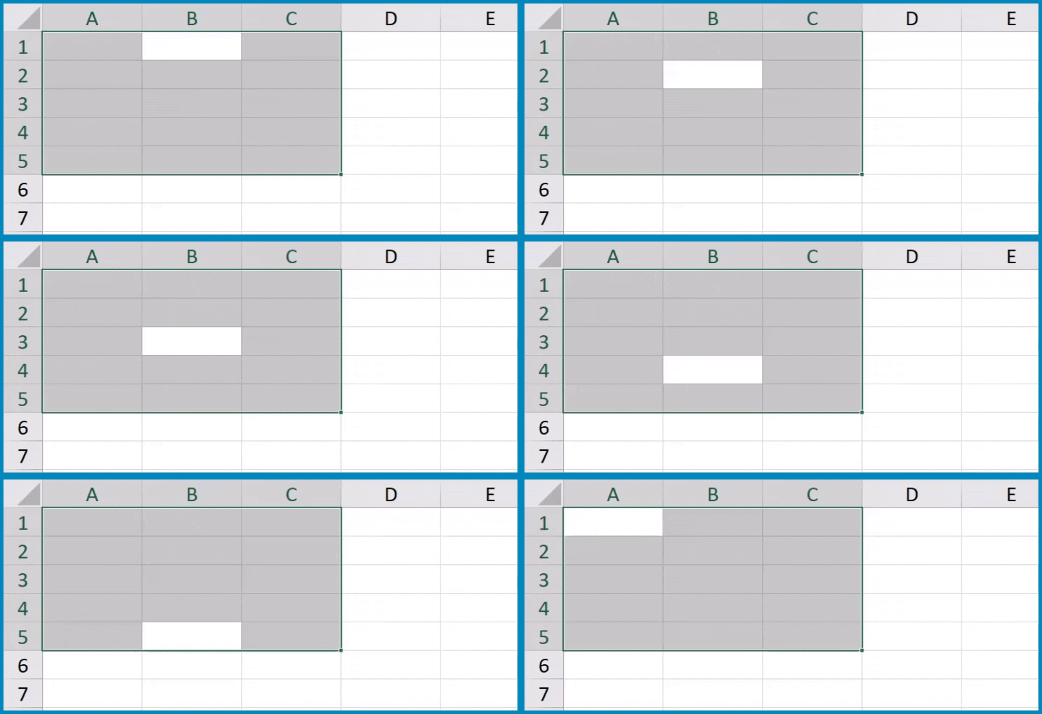
If you know you wish to restrict the data to a set range of rows and columns, you can pre-select the range. By doing so, repeated pressing of the Tab key will confine the cell selections to the pre-selected range.
Formatting Data (Let’s make this pretty!)
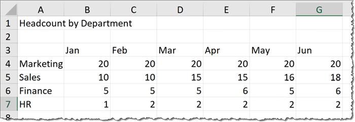
We have a set of data where department headcounts are displayed by month.
Attractive Titles
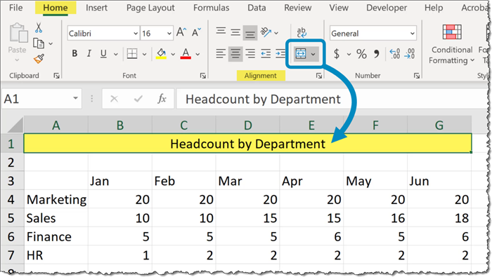
To make the report more attractive, we begin by centering the heading between columns A and G. This is accomplished by selecting the cells you wish to center across (A1 through G1) and press the Merged & Center button.
Resizing Multiple Columns
If you wish to tighten up the space used by the monthly columns (B through G), select the column headings for columns B through G, then double-click one of the highlighted column heading dividers (remember Auto Fit?).
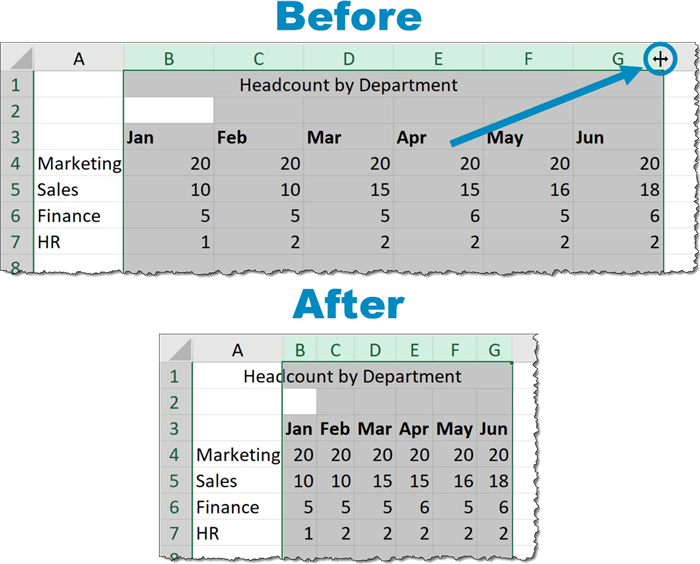
If this is too tight, you can manually expand one of the selected column heading dividers and manually resize to the desired width. This new size will be applied to all selected columns, providing a professional, uniformed look.
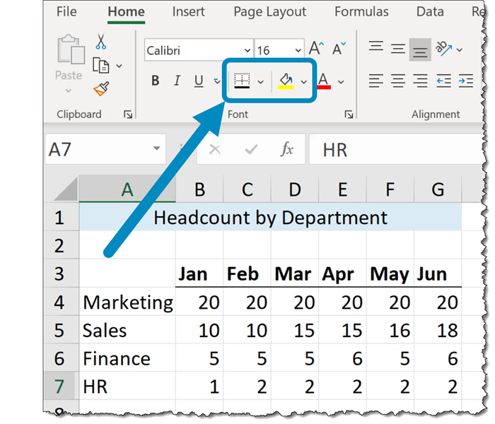
Adding Colors and Borders
With the Month cells selected, we can apply any traditional cosmetic changes to the cells, like font style, font size, font color, alignment, etc.
We can also add borders and fill colors to the cells using the Borders and Fill Color features.
Moving Rows (the COOL Way)
Suppose you want to move the order of the Departments in our table above.
Most users would perform the following steps:
- Insert a blank row where they want the data to be moved to
- Select the data to be moved
- Invoke a Cut action
- Select the newly inserted empty row
- Invoke a Paste action (or right-click -> “Insert Cut Cells”)
Although that works, it’s not exactly a crowd-pleasing party trick. Try this instead:
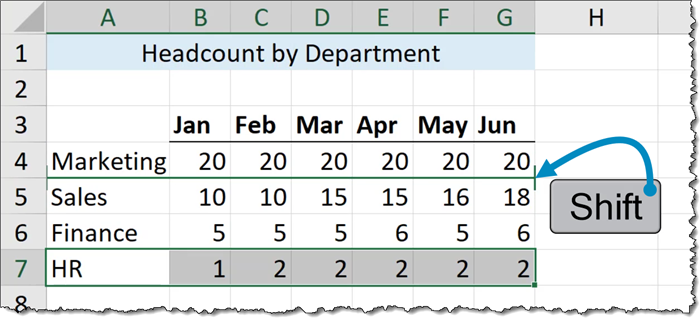
- Select the cells you wish to relocate (ex: A7 through G7).
- Click and hold the border of the highlighted cells (stay away from the Fill Series handle).
- While you drag up or down, press the SHIFT This will reveal a thick green line that indicates the drop location.
Speedy Formatting Trick
If you have a cell that has a certain style (i.e., color, size, font, etc.) and you want all of those same settings applied to other cells, you can use the Format Painter to copy and paste the look of a cell without carrying over the data.
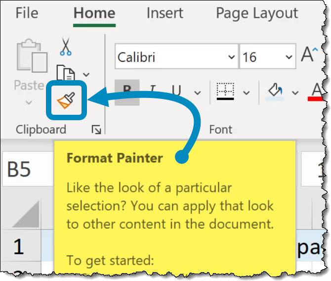
Select the cell that has the style you wish to replicate, click the Format Painter button, then click the cell to which you want to apply the style.
Pro Tip: If you need to apply the style to many cells that may not be in a consecutive arrangement, double-click the Format Painter button to lock it into an “on” state. Select all the needed cells, then click the Format Painter when you’re finished to deactivate the feature or press the ESC key.
Creating Your First Calculations (Adding Values)
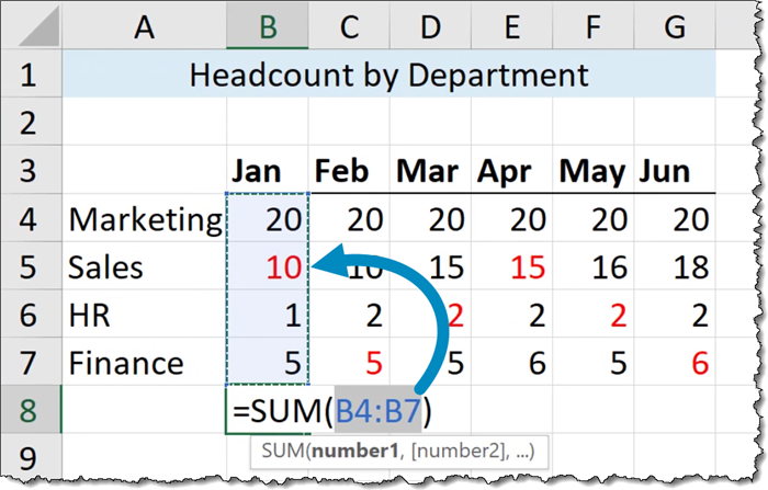
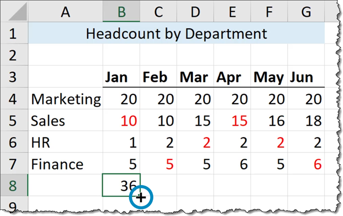
If we want to get the monthly totals for all Departments, select the cell below the “Jan” values (cell B8) and press the AutoSum button (or press the ALT-Equals sign) located in the upper-right corner of the Home ribbon.

This will create a formula that uses the SUM function. The formula will attempt to determine the extent of the data. We can easily verify the selection by examining the Marquee (moving dotted line surrounding the selected cells).
Repeating Formulas
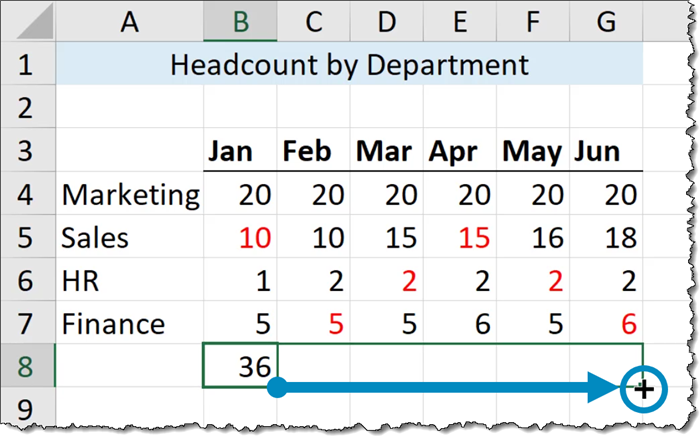
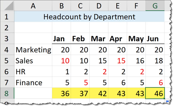
If you need to create the same type of formulas for the remaining months, perform the following steps:
- Select the cell with the formula you wish to repeat.
- Place the mouse pointer (thick, white plus symbol) over the Fill Series You should see a thin, black plus symbol.
- Drag the Fill Series handle to the right across the remaining columns of calculations.
Closing Thoughts
Knowing a few of the most used features of Excel will give you the confidence to want to learn more.
The journey to learn Excel is endless, but as with all journeys, it must begin with a few small steps.
Today you walk, tomorrow you run, and soon you will fly.
Leila Gharani
I'm a 6x Microsoft MVP with over 15 years of experience implementing and professionals on Management Information Systems of different sizes and nature.
My background is Masters in Economics, Economist, Consultant, Oracle HFM Accounting Systems Expert, SAP BW Project Manager. My passion is teaching, experimenting and sharing. I am also addicted to learning and enjoy taking online courses on a variety of topics.


