#1: Creating External Links Without Knowing
Nobody wants to reinvent the wheel. Therefore, it’s common to copy portions of an existing spreadsheet into a different spreadsheet.
Unfortunately, this is where you can fall into a trap.
Take the following workbook named “Start.xlsx” as an example. We have two sheets named “Calculation” and “Master”.
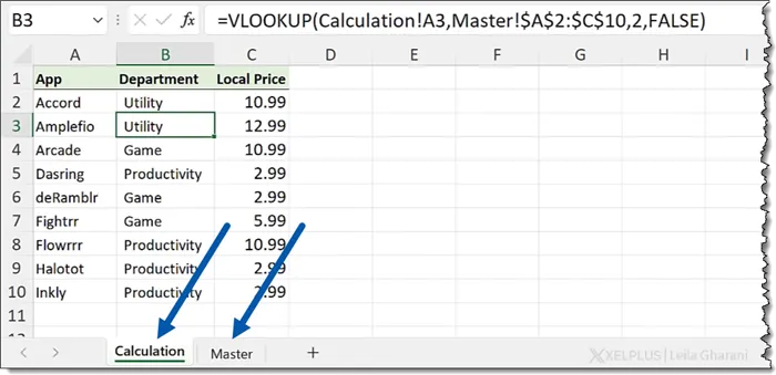
Notice that the “Calculation” sheet has formulas that reference the “Master” sheet.

If we were to copy the “Calculation” sheet to a new workbook named “LocalFile.xlsx” using the following steps:
- Right-click the “Calculation” sheet.
- Select “Move or Copy”.
- Select “xlsx” as the “To Book” option.
- Check the box labeled “Create a Copy”.
- Click OK.
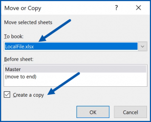
We can see in one of the formulas in the destination file that the formulas do not continue to point to a sheet named “Master”, rather they are attempting to return to the file named “Start.xlsx” and read that file’s “Master” sheet.

Assuming this pointer to the original file is undesirable, we need to perform one of two actions:
- Redirect the file pointers in the formulas to use the new/destination file, or
- Break the links and remove the formulas while leaving the formula results.
Redirecting Formula Pointers
The odds are good that you are not being paid by the keystroke, so manually updating each formula to point to the new file is not an option.
We can redirect all the original formula pointers from the “Master” sheet of the original file (“Start.xlsx”) to the “Master” sheet of the new file (“LocalFile.xlsx”).
- Select Data (tab) -> Queries & Connections (group) -> Edit Links.
- In the “Edit Links” dialog box, click the link(s) that point to the original file.
- Click the Change Source
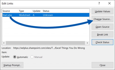
- Browse and select the new file (ex: “LocalFile.xlsx”).
- Click OK.
All formulas that originally pointed to the “Start.xlsx” file are now pointing to the new “LocalFile.xlsx” file.

Breaking the Links
If you do not need to maintain the dynamic nature of the formulas, rather you just need the results as last calculated, you can break the links by performing the following steps:
- Select Data (tab) -> Queries & Connections (group) -> Edit Links.
- In the “Edit Links” dialog box, click the link(s) that point to the original file.
- Click the Break Link
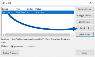
- Click OK.
Notice that the last calculated value remains in the cell without the original formula.
Featured Course
Excel Essentials for the Real World

#2: Manually Adjusting Text in Cells
This one is more of a productivity tip than an observation of something you’re doing wrong.
Suppose you are including instructions in your worksheet and the text is getting a bit lengthy.

The thing NOT to do is to break the text into smaller pieces and place each piece in a separate cell.
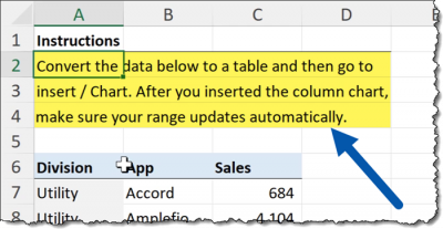
You may think you have won the day, but the moment you must add, remove, or edit the text in any way, you’ll likely have to rework the entire paragraph based on the new edits.
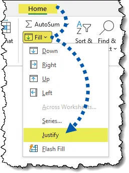
Instead, select the range of cells you want the text to occupy then click Home (tab) -> Editing (group) -> Fill -> Justify.
Everything now flows within the selected range.
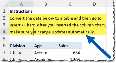
If you need to restore the text to a single line, select as many cells on a single line as you think are needed to contain the text, then repeat the Home (tab) -> Editing (group) -> Fill -> Justify step.
Featured Course
Black Belt Excel Package

#3: Merging Cells Instead of Centering Text
Every tool has its place and time.
Merging cells may be useful at the top of a report, but you shouldn’t merge cells in the middle of your data.
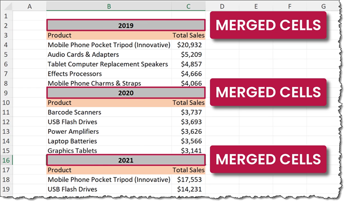
This is a poor place for merging cells. Many negative behaviors crop up when working with a mixture of merged and non-merged cells.
In the above image, if you tried to select all of the values in column C, the system would automatically extend the selection range to include column B, since the merged cells exist in both columns.
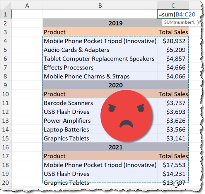
There are many crude and tedious ways to try and overcome this, but why bother when you can just correct the issue by merging cells in a non-destructive manner?
Using “Center Across Selection”
Your new best friend when it comes to merging cells is called Center Across Selection.
The way you use this superior technique is:
- Select the cells you wish to center the text across.

- Click the “deep dive” icon in the Alignment group on the Home ribbon (or press CTRL-1).
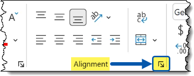
- On the Alignment tab, select Center Across Columns from the Text Alignment -> Horizontal option.
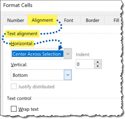
This will produce the same look like the previous, inferior method while retaining the individuality of each selected cell.
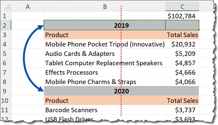
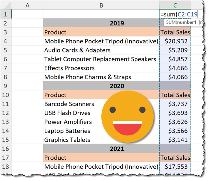
Selecting cells in column C is now contained to column C, no longer intruding into column B.
Bonus Tip #1: Quickly Access the Alignment Dialog Box
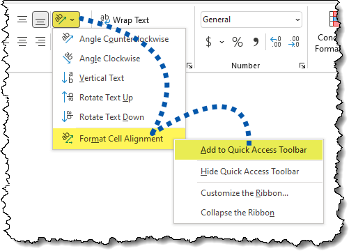
If you find yourself using the alignment controls regularly, you can gain access to these controls more easily by adding a launch button on the Quick Access Toolbar.
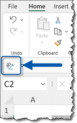
An easy way to add this button to your Quick Access Toolbar is to perform the following steps:
- Click Home (tab) -> Alignment (group) -> Orientation
- Right-click the bottom option labeled Format Cell Alignment.
- Click Add to Quick Access Toolbar.
Bonus Tip #2: Locate All Merged Cells on a Worksheet
If you are unsure which cells have been merged (especially difficult to see when gridlines have been turned off), you can locate all merged cells with the aid of the FIND feature. Perform the following steps:
- Press CTRL-F to open the Find dialog box.
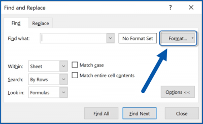
- Click the button labeled “Format…” in the upper-right of the Find and Replace dialog box.
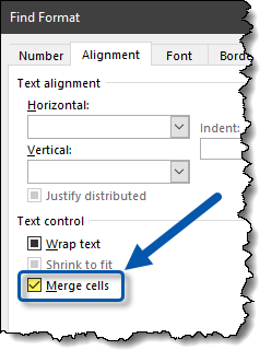
- On the Alignment tab, place a check in the box labeled Merge Cells.
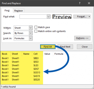
- Repeatedly click Find Next to “step” through all discovered cell merges or click Find All to display a list of all cell merge locations.
#4: Poor File Structure
It is all too common for users to place all their report elements on a single sheet. The sheet will contain:
- The raw data
- The intermediate calculations
- The aggregations used to answer key questions about the data
- Visualizations (e., charts, graphs, KPIs, etc.)
- Instructions for users regarding the operation of the report
A better approach is to store these elements on separate sheets.

Since most users will not require access to the supporting pages (ex: raw data & calculations), these sheets can be hidden. This greatly reduces file corruption as the temptation to interact with these elements is removed.
Featured Course
Power Excel Bundle

#5: Hiding Rows & Columns In the Wrong Places
Hiding rows and columns is a great skill. Often we are required to create spreadsheet elements that are necessary for proper operation, but we don’t want them to appear on the screen or the printout.
The downside to hiding things is that they can interfere with other users who are not aware of their existence.
Take the following worksheet as an example.
We have a list of sales, and we want to get a quick total at the bottom of column C.
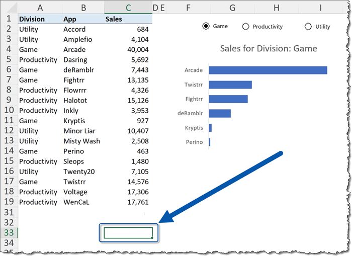
The user writes a quick SUM formula that targets all the cells above their current location.
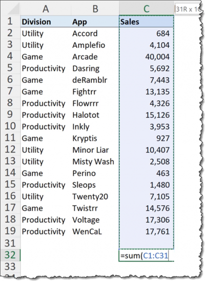
When they hit ENTER, they receive an answer, but they don’t realize that the answer is incorrect.
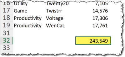
But why is the answer wrong?
It’s subtle but notice that rows 20-30 have been hidden.
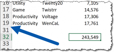
Unhiding rows 20-30 reveals values that were created to service the chart in column F.
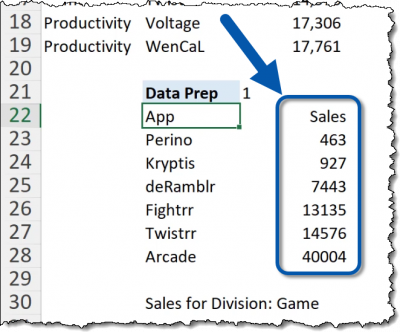
Most users aren’t going to notice the skipped row numbers; and honestly, why should you expect them to?
A way to hide the rows and draw attention to their hidden state is to use the GROUP feature.
By selecting rows 20-30, then pressing

You can also activate the GROUP feature by clicking Data (tab) -> Outline (group) -> Group / Ungroup.
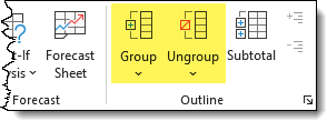
NOTE: You can ungroup rows and columns using the UNGROUP button on the Data tab or press

The dots and lines next to the grouped rows that lead to the big “minus” button indicate that the rows have been grouped.
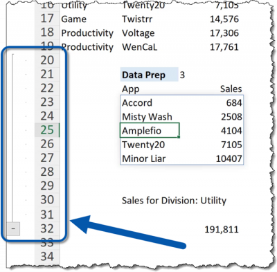
Clicking the “minus” to hide the rows transforms the button into a “plus” button.

This makes it a bit more obvious that rows have been hidden.
PRO TIP: This leads back to the previous topic about separating workbook elements into different sheets. Calculations that feed charts should be stored on a sheet independent of the raw data sheet. This would make this entire scenario moot. But if you must store your data in this manner, you can at least make it more obvious using grouped rows.
#6: Hardcoding Numbers in Formulas
A common “mistake” users make is hardcoding values into formulas that are likely to change.
For example, we’re working in a financial model where certain values are used in multi-year calculations, such as this discount of 8% used in years 2021 and beyond.
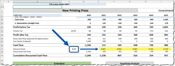
When investigating why the results don’t seem to calculate correctly, it’s discovered that the 8% in cell C51 is not being referenced in the succeeding formulas. Rather, it a value of 6% has been hardcoded into the formula(s).
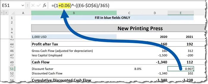
The formula should have been typed as…
=(1 + $C$51 ) ^ - ( (etc…This way, changing the percentage in cell C51 would automatically flow to the successive formulas.
We can’t expect the user to update every formula that may use the percentage as part of its calculation.
Locating Dependent Formulas
We can quickly and easily discover every cell that is using the value in cell C51 using Excel’s Auditing Tools.
- Click the cell you want to check for dependencies (ex: cell C51).
- Select Formulas (tab) -> Formula Auditing (group) -> Trace Dependents.

This will display arrows to every cell on the sheet that uses cell C51’s value/result as a part of its calculation.
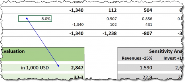
As we can see, the value of cell C51 is used in cell D59 but not in cells E51, F51, G51, etc.
This discovery can be performed in reverse.
If we want to see if cell C51’s value is used in cell E51, click in cell E51, then press the Trace Precedents button.

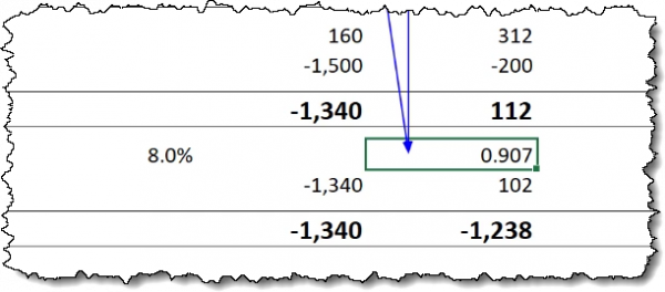
We see that there are some cells above that are “feeding” cell E51, but cell C51 is not one of them.
You can remove the arrows from the screen by clicking Remove Arrows.
PRO TIP: Each time you click the Trace Precedents or Trace Dependents buttons, the system will step forwards or backward through the data flow displaying arrows to each successive step.
#7: Not Using Tables
Tables are data arranged where the columns represent categories and the rows represent transactions/records.
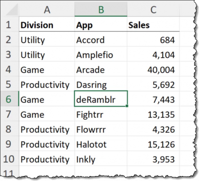
Entering the data in this way, we create what many users refer to as a “plain” table.
You can create many useful objects from this “plain” table, such as:
- Charts
- Pivot Tables
- Pivot Charts
- Formulas to enhance the original data
- Formatting to enhance the data
There is a major drawback to creating such objects from “plain” tables. The addition or removal of rows or columns in the “plain” table requires manual intervention to update the objects based on that table.
If you’re working with only one or two charts, this is not a big deal. Imagine working with dozens or hundreds of visualizations based on the data.
Upgrading a “Plain” Table to a Proper Excel Table
You can easily upgrade a “plain” table to a proper Excel Table by selecting the data and clicking Home (tab) -> Styles (group) -> Format as Table.
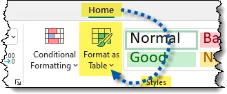
Or by pressing…

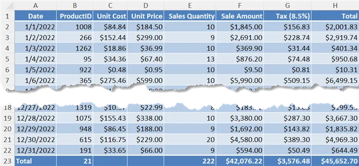
Once upgraded to a proper Excel Table, you can choose from a variety of pre-built color schemes and visual enhancements, such as:
- Row banding
- Column banding
- First column accenting
- Last column accenting
- Differently colored header row
- Differently colored total row
You can also leverage many useful behaviors exclusive to proper Excel Tables:
- Automatic color management that is immune to sorting, filtering, adding, removing rows and columns
- Easily created aggregations via dropdown lists
- Automatic header row “snapping” when scrolling through large tables
- Formulas that utilize structured references instead of traditional cell references
- Automatic data formatting (ex: Currency style, Comma style, Date style, etc.)
- Dynamic range references in external calculations
- Automatic formula creation when adding new rows where columns contain formulas
- Add or delete table rows without modifying data on the same row to the side of the table
- Automatic updating of all charts based on the table’s data
- Easily filter and sort using built-in header controls or right-click menus
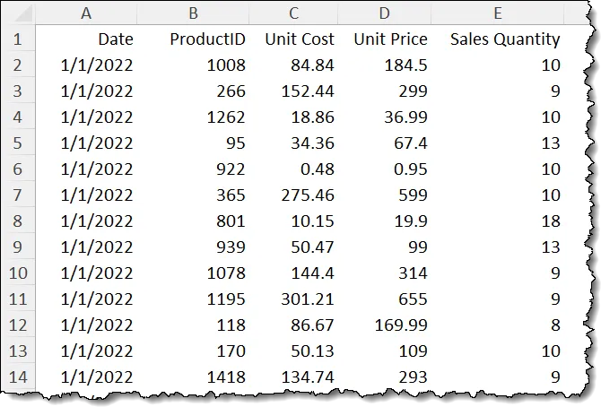
Can be transformed into this:
Cheat Sheet
Download the handy Cheat Sheet summarizing all the tips:
Leila Gharani
I'm a 6x Microsoft MVP with over 15 years of experience implementing and professionals on Management Information Systems of different sizes and nature.
My background is Masters in Economics, Economist, Consultant, Oracle HFM Accounting Systems Expert, SAP BW Project Manager. My passion is teaching, experimenting and sharing. I am also addicted to learning and enjoy taking online courses on a variety of topics.


