Creating (Recording) a Macro
The first step in any macro endeavor is to create the macro.
Macros are small computer programs that are executed when you click a button or press a keyboard shortcut. These little programs are written in a language called Visual Basic for Applications, or “VBA” for short.
Now don’t click away so fast. You can create and reap the benefit of macros without ever seeing a single character of VBA code. Excel has a super-convenient way of creating macros that only requires that you do what you already know how to do.
In other words, if you can perform a set of steps to accomplish a goal in Excel, you only need to learn a few more steps to turn those steps into an automated process.
If you can record a video on your phone (and I know you can), you have the skills to create macros.
Excel provides a tool called the Macro Recorder, whereby you press a record button, then perform the steps you would normally perform to meet the goal followed by the pressing of a “stop” button.
Once the steps have been recorded, you can click a button to execute all the recorded steps at lighting speed (or at least as fast as your computer can execute the steps.)
Imagine yourself as a famous singer (unless you are one.) What if the only time your songs could be heard is when you sing those songs live. You’d probably grow tired of singing the same song(s) over and over.
Then someone invents this magical device that allows you to record your song and play it back as many times as you like without any effort on your part. You could even send the song to others so they could hear it without you even being there.
That’s the magic of macros.
Let’s look at an example.
Creating a Chart from Daily Report Data
Suppose we receive a daily report of data that we are required to turn into a specific type of chart with various features and customizations.
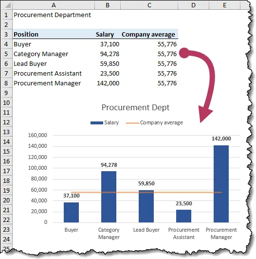
The catch with the data is that some days there are more rows of data than other days.
We want to make the process of chart creation completely dynamic, so we don’t have to create the chart from scratch every time we receive a new day’s file.
Starting the Macro Recorder
To record a macro, click either the “Record Macro” button located in the lower-left corner of the Excel window…
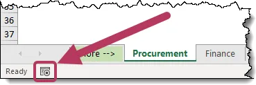
… or select View (tab) -> Macros -> Record Macro.

Adding the Developer Ribbon
If you want to record macros the way the “cool kids” do it, you can activate a special ribbon known as the Developer ribbon. This ribbon contains the various tools for creating and editing macros.
To activate the Developer ribbon:
- Right-click on any visible tab and select “Customize the Ribbon…”.
- In the Excel Options dialog box, place a check next to the “Developer” entry on the right panel of options, then click OK.
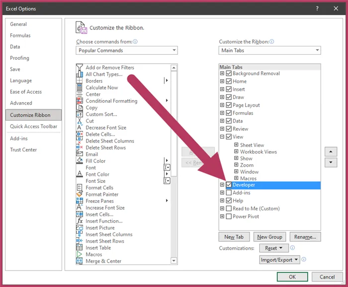
You now have access to all the cool toys.

Recording a Macro
PRO TIP: Just like the “record a song” analogy earlier, you want to think through all the steps you are going to perform before creating the recording. Any unwanted steps performed during the recording process will become part of the playback procedure. If you happen to make a mistake during the recording process, you can always delete the macro and try again. (Do you think Lady Gaga sang “Bad Romance” perfectly the first time?)
Using one of the methods described above, start the macro recorder. The following dialog box appears.
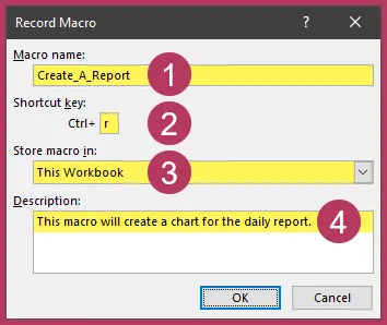
- Each macro requires a name. The name cannot contain any spaces and must be unique to this file. We will use “Create_A_Report” as our macro name.
- You can assign a shortcut key to the macro for easier execution, such as CTRL-r.
- You can store the macro in the file or the Personal Macro Workbook.
- You can add a description to the macro for documentation purposes.
Click OK to start the recorder.
Every click and everything typed, edited, or deleted will be recorded.
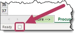
Notice the icon in the lower-left of the Excel window has changed from a “record” button to a “stop” button.
Let’s perform the following steps to creator our chart that will be reproduced by the “Create_A_Report” macro:
- Click in cell A3 to establish the upper-left corner of the data. NOTE: Do NOT highlight the data range. If you do, you will force the macro to always select the defined range. If later you have data that goes beyond that range, it will be ignored. If later you have less data, you will end up selecting too many cells and have empty areas in your report.
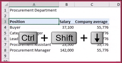
- To properly select the data range so it will be dynamic during future executions, press CTRL-Shift-Down arrow then press CTRL-Shift-Right Arrow.
- To create the chart, select Insert (tab) -> Charts (group) -> Combo Chart.

A new combo chart has been inserted into the file.
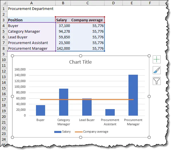
WARNING: Do NOT click away from the chart and reselect it. If you do, the chart’s name (ex: “Chart2”) will be hard-coded into the macro which will cause a failure later since the next chart will be a different name like “Chart3”. If you leave the chart selected, the macro code will refer to it as the “active chart” without any specific name.
- Perform any cosmetic changes to the chart you like, such as changing bar colors, add data labels, customize the legend, customize the title, etc.
- Click the “Stop” button (bottom-left) to stop the recorder.
Featured Course
Unlock Excel VBA & Excel Macros

Testing the Macro on a Different Data Set
To test the macro, select a sheet of new data and launch the macro recording from above.
Macros can be launched in many different ways:
- Pressing the keyboard shortcut assigned to the macro during the recording process (ex: CTRL-r).
- Selecting View (tab) -> Macros -> View Macros -> select the macro -> Run.
- Selecting Developer (tab) -> Code (group) -> Macros -> select the macro -> Run.
More exotic users may even assign macros to shapes and images that when clicked will execute the macro. Those are the REALLY cool kids.
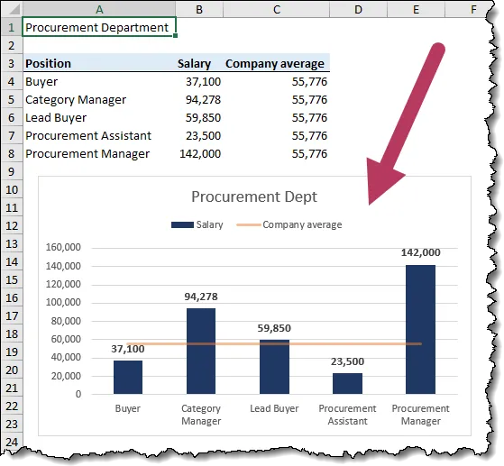
Notice that in just a couple of clicks or the press of a keyboard shortcut we have a perfect chart of the new data.

Well, almost perfect.
The chart’s title was hard-coded to display “Procurement Dept”. We want this to be dynamic and display the text located in cell A1 of the selected sheet.
This change needs to be made in the VBA code as it can’t be recorded dynamically.
Opening the VBA Editor to Reveal the Code
To open the VBA Editor, either press CTRL-F11 or click Developer (tab) -> Code (group) -> Visual Basic.
The VBA Editor will open to display the recorded steps as code. If you don’t see any code in the window, you will need to double-click one of the entries labeled “ModuleX” on the left side of the screen in the Project Explorer window.

Scrolling down through the code we see a line of code towards the bottom that reads…
Selection.Caption = “Procurement Dept”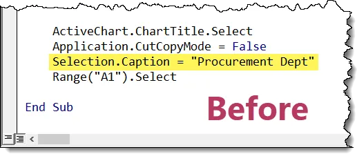
We need to change this to read…
Selection.Caption = Range(“A1”).Value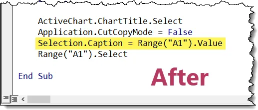
I said you can use macros without ever working with the VBA code, but it’s a good idea to learn a little bit of code so you can perform basic maintenance and changes to the macro without having to recreate the entire macro.
Bulletproofing the Macro
As it stands, our macro assumes that the sheet it is executed against has data. If it does not, the macro will result in an error.
We can build in a bit of pre-testing of the sheet to determine if the sheet is empty or has data. This way, we can inform the user of the situation and not attempt chart generation. This will be a more elegant and professional way to handle the situation.
This type of testing cannot be created via the macro recorder; it must be written manually.
At the top of the code, enter the following text:
If Range(“A3”).Value <> “Position” or Range(“A4”).Value = “” Then
Exit Sub
Else
Scroll to the bottom of the code text and enter the following:
End If
If you would like to learn more about the VBA language and improve your skills at creating amazingly flexible macros, check out my VBA course using the link below.
Unlock Excel VBA & Excel Macros – XelPlus.com
Testing the Updated Code
To test the macro to ensure the chart title is dynamic and the empty sheet detection works, select a different sheet of data and run the macro.
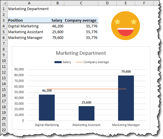
Notice that the chart title mimics the text located in cell A1.
If we select an empty sheet and run the macro, nothing happens because the sheet contains no data.
Saving Your File That Contains Macros
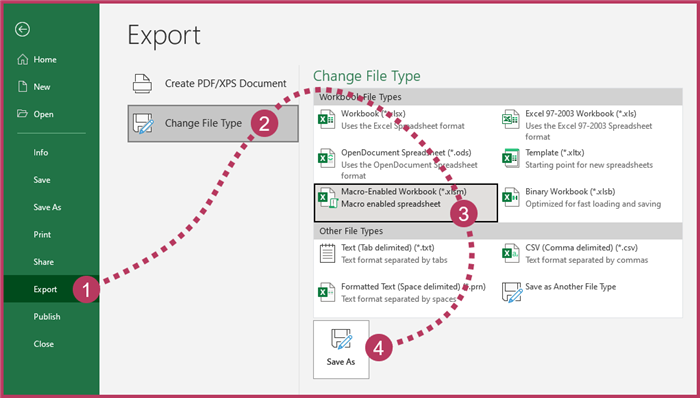
When you save your file that contains any macros, you cannot save the file with a traditional .XLSX file extension. The file must be saved with an .XLSM file extension to denote a macro-enabled file.
If you opt to save the file as a traditional .XLSX file, any macros and their VBA code will be discarded.
To save the file without losing your macros, perform the following steps:
- In the Backstage (click File), click Export
- Click “Change File Type”
- Click “Macro-Enabled Workbook (*.xlsm)”
- Click “Save As”
Save the file to a location and with a name of your choosing.
Working with Relative References in Macros
VBA can work with relative references in Excel. If you’d like to see an example of such a scenario, click the following link for a post & video demonstration.
Move Data Sheet to Sheet
Practice Workbook
Feel free to Download the Workbook HERE.

Leila Gharani
I'm a 6x Microsoft MVP with over 15 years of experience implementing and professionals on Management Information Systems of different sizes and nature.
My background is Masters in Economics, Economist, Consultant, Oracle HFM Accounting Systems Expert, SAP BW Project Manager. My passion is teaching, experimenting and sharing. I am also addicted to learning and enjoy taking online courses on a variety of topics.


