Parsing (i.e., splitting) data is typically based on the presence of a special character known as a delimiter in the data.
Delimiters mark the end of one piece of information and the beginning of another piece. The most encountered text delimiters are the comma and the tab, but other characters like the colon, semi-colon, and slashes are not too uncommon.
If your data consistently uses the same delimiter throughout its scope, certain tools can be used without much effort, like the “Text to Columns” tool found on the Data tab. You can even think of the new TEXTSPLIT function as the formula version of “Text to Columns”.
The problem with a tool like “Text to Columns” is that it’s not dynamic; the results do not update when the source material changes.
If you tried to write your own custom formula to deal with splitting text, mixed delimiters and data of varying lengths can cause problems. The greater the variety in the data, the more complex the formula tends to be to deal with the variety.
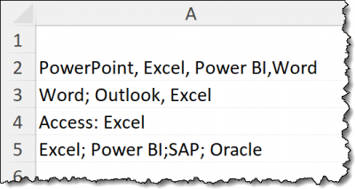
In the above image, notice some of the issues that need to be addressed when parsing the application names into separate cells:
- A mixture of delimiters; commas, semi-colons, and colons.
- A varying number of applications per row.
- Some delimiters are followed by a space while other delimiters lack a space.
To deal with these inconsistencies in the data would require quite an elaborate formula to produce a reliable result.
TEXTSPLIT will not only deal with these issues but when paired up with a few other functions can achieve some truly monumental transformations.
The Syntax of the TEXTSPLIT Function
The TEXTSPLIT function has the following syntax:
=TEXTSPLIT(text, col_delimiter, [row_delimiter], [ignore_empty], [pad_with])The arguments for TEXTSPLIT are:
- text – The text you want to split. (Required)
- col_delimiter – One or more characters that specify where to spill the text across columns. (Required)
- row_delimiter – One or more characters that specify where to spill the text down rows. (Optional)
- ignore_empty – Specify TRUE to create an empty cell when two delimiters are consecutive. Defaults to FALSE, which means don’t create an empty cell. (Optional)
- pad_with – The value with which to pad. The default is #N/A. (Optional)
Let’s look at some examples of what TEXTSPLIT can do for you.
Featured Course
Black Belt Excel Package

TEXTSPLIT Basics
Using the example data seen previously, we want to split the listed skills into separate cells.

Starting with the first row in the data, we can write a TEXTSPLIT function in the following way:
=TEXTSPLIT(A2, “,”)
“A2” is the cell holding the combined data, and the “,” is the delimiter separating the elements.
The result may appear to be a resounding success, but if you look more closely, you’ll see a small issue.
The spaces that followed the commas are now preceding the parsed text.

We have two ways we can deal with this issue:
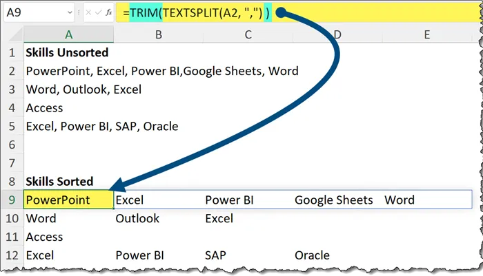
- Nest the TEXTSPLIT function within a TRIM function to remove the extraneous leading spaces, or
=TRIM(TEXTSPLIT(A2, “,”) )- Modify the defined delimiter to be a “comma-space” delimiter description.
=TEXTSPLIT(A2, “, ”)
Repeating the Formula Across Cells
We’ve solved the parsing problem for the first cell of data but look what happens when we repeat the formula down to other cells.

This doesn’t work very well because of the use of differing delimiters; colons and semi-colons used with commas.
The good news is that TEXTSPLIT can be supplied with multiple delimiters by which to parse the data.
The catch is that when supplying multiple delimiters, you must separate each delimiter with a comma and enclose the entire list of delimiters within a set of curly braces.
=TEXTSPLIT(A2, { “,”, “:”, “;” } )
You could even front-load the list of delimiters that you think you may encounter, just to make it more future-proof.
Featured Course
Excel Essentials for the Real World

Skipping Blanks in TEXTSPLIT
Below we have a list of names that we want to split into first and last names.
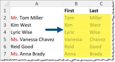
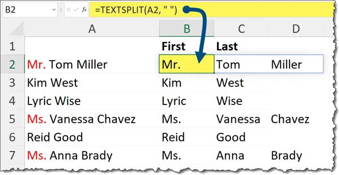
The issue here is the presence of the title “Mr.” and “Ms.”. If we split the text using the space as the delimiter, we end up with the following undesirable results.
In addition to single-character delimiters, we can use text strings to represent delimiters.
Let’s use the titles themselves as delimiters to separate the text.
=TEXTSPLIT(A2, { " ", "Mr. ", "Ms. " } )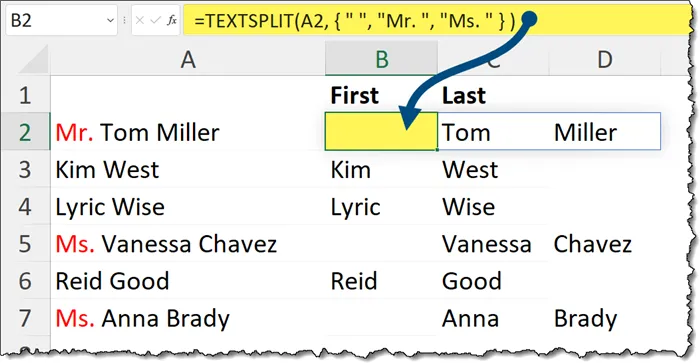
This is getting better, but we have introduced spaces where the titles used to be.
The TEXTSPLIT function includes an argument called [ignore_empty] that keeps this issue from occurring.
By adding “TRUE” to the [ignore_empty] argument, we can ignore the introduction of spaces in the result.
=TEXTSPLIT(A2,{ " ", "Mr. ", "Ms. " }, , TRUE)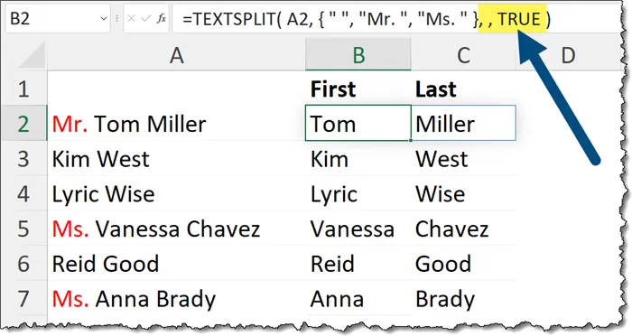
TEXTSPLIT to Columns and Rows
Splitting text from a single cell into multiple rows and columns is simple with TEXTSPLIT.
Take a look at the following data that is in a single cell that we need to split into a name column and a salary column.
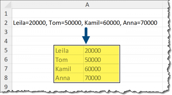
We can use the equals sign to separate the names and salaries into separate columns while using the comma-space to separate the data into rows.
=TEXTSPLIT(A2, "=", ", " )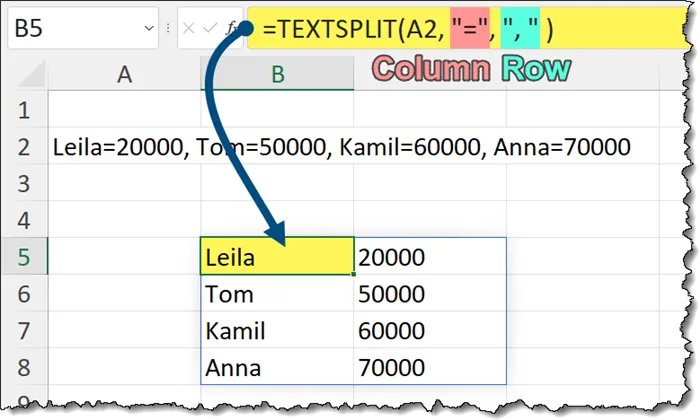
Featured Course
Master NEW Excel Functions in Office 365 & Office 2021

TEXTSPLIT, SORT & Stitch Back (TEXTJOIN)
Let’s try something really cool.
We have the list from earlier of application skills in a combined, unsorted manner, and we wish to have them in a combined, sorted manner.
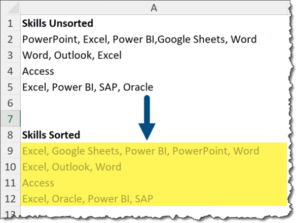
There isn’t a single function solution to produce this result, but we can achieve the goal in three simple steps:
- Split the text into separate cells using the TEXTSPLIT
- Sort the separated results using the SORT
- Recombine the individual elements back into a single cell using the TEXTJOIN
Step 1 – Split the text
We’ll start by utilizing our new favorite function, TEXTSPLIT, to separate the skills into cells.
=TEXTSPLIT(A2, “,”)NOTE: I’ve filled the formula down to the adjacent rows to apply the formula to the remainder of the list. I’ll be doing this for the following steps as well.
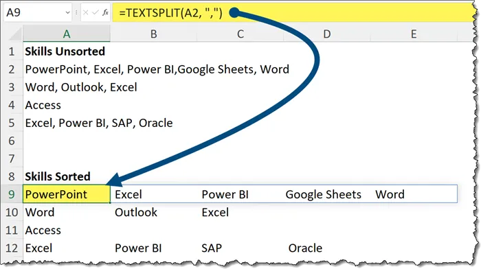
Because some (not all) of the comma delimiters have spaces following them, we’ll slip in a little TRIM function to remove the extraneous spaces.
Step 2 – Sort the Separated Skills
We can easily sort the skills by nesting the TRIM/TEXTSPLIT functions inside a SORT function.
=SORT(TRIM(TEXTSPLIT(A2, ",") ), , , TRUE )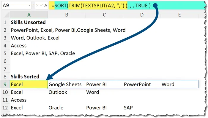
In the SORT function, we had to skip the 2nd and 3rd arguments ([sort_index] and [sort_order]) to be able to define the 4th argument, [by_col]. The TRUE tells the SORT function to sort the data by columns as opposed to by rows which is the default behavior.
Step 3 – Combine the Results into a Single Cell
The final step is to use a TEXTJOIN function to combine the separate cells into a single cell.
=TEXTJOIN(", ", TRUE, SORT(TRIM(TEXTSPLIT(A2, ",") ), , , TRUE ) )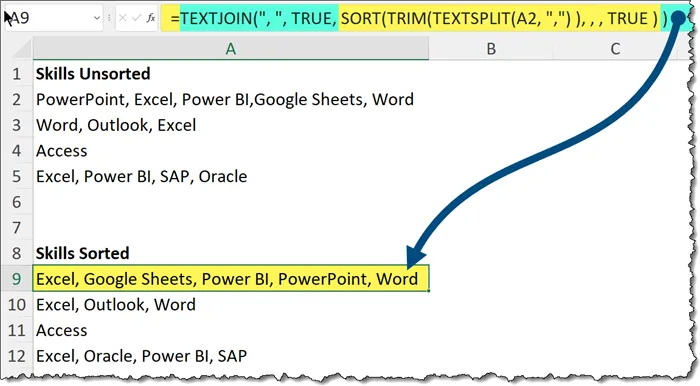
The TEXTJOIN function uses a comma-space as the delimiter, and the TRUE tells TEXTJOIN to ignore any empty cells in our data. As we didn’t have any empty cells, TRUE or FALSE would yield the same result.
Only Limited by Your Imagination
The TEXTSPLIT function is one of those functions that allow you to exercise your creativity to solve what used to be challenging problems.
Combine TEXTSPLIT with other functions to both compliment and enhance TEXTSPLIT’s abilities.
Your days of writing complicated solutions to simple problems are coming to a fast close.
Practice Workbook
Feel free to Download the Workbook HERE.

Leila Gharani
I'm a 6x Microsoft MVP with over 15 years of experience implementing and professionals on Management Information Systems of different sizes and nature.
My background is Masters in Economics, Economist, Consultant, Oracle HFM Accounting Systems Expert, SAP BW Project Manager. My passion is teaching, experimenting and sharing. I am also addicted to learning and enjoy taking online courses on a variety of topics.


