Excel provides many options for sorting data. Depending on the data, sorting can be performed using the following strategies:
- If your data is text, you can sort alphabetically in either an ascending (A to Z) or descending (Z to A) fashion.
- If your data are values (numbers), you can sort numerically as ascending (smallest to largest) or descending (largest to smallest).
- If your data are dates, you can sort chronologically in an ascending (oldest to newest) or descending (newest to oldest) fashion.
Excel also provides a method for sorting based on a user-defined custom list. This list would allow you to define the exact order you wish items to appear (more on this later.)
If you are using Conditional Formatting (or manually formatting), you can sort by cell color, font color, and even by icon when using icon sets.
Sorting Basics
In the below example, we have data recorded by Division, Region, Apps, and Revenue. If we want to determine which Apps have the highest revenue, we can click ANYWHERE in the Revenue column’s data (no need to highlight the entire column or entire table like we did in the “old days”) and then right-click and choose Sort and then choose Sort Largest to Smallest.
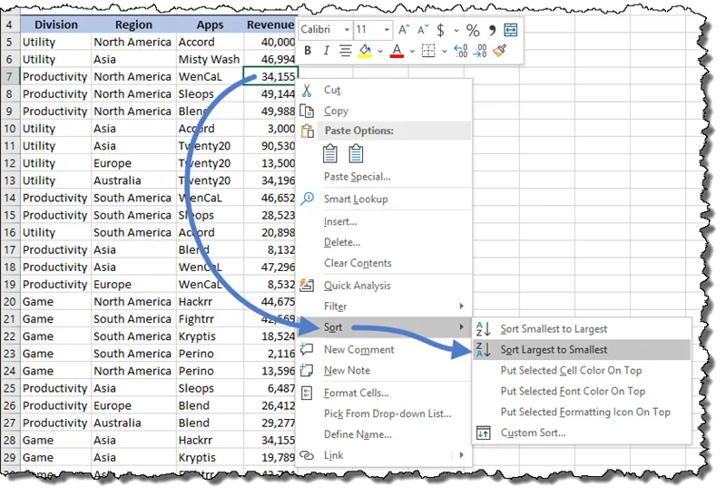
Excel is smart enough to recognize that all the data on the same row as a Revenue value is associated with that value and should move wherever the Revenue moves. Excel is also smart enough to understand that the first row of the data is a header row and should not be moved with the other rows.
TIP: If you are unsure as to what Excel “sees” as the data range, click anywhere in the table and press CTRL-A. This will highlight the data considered to be part of the selected table.
If you wish to sort by one of the other columns in the table, right-click on any cell in the desired column and choose Sort and then choose the sort logic that best fits your need.
Featured Course
Excel Essentials for the Real World

Problem with Adjacent Data
If you have data that is directly next to the table to be sorted, and you do not want that adjacent data to be included in the sort procedure, you must highlight the entire table, including headers, and then select Custom Sort.
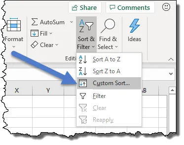
The Custom Sort feature can be accessed a variety of different ways. Some of the more common ways are to select the Home ribbon and then select Sort & Filter and then choose Custom Sort.
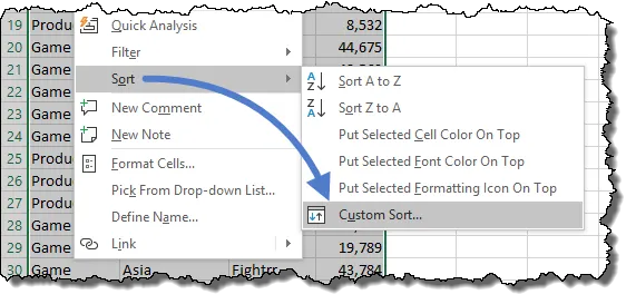
Or, right-click the highlighted table and choose Sort and then choose Custom Sort.
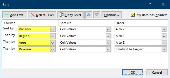
The Sort dialog box gives you full control over how you wish to sort your data. You can sort by multiple criteria (levels) and inform Excel as to whether your table has a header row or not.
Custom Lists
Suppose that when we sort the Division column alphabetically in either ascending or descending fashion, we don’t arrive at the order we wish it to be. Suppose we wish the Divisions to be listed as follows:
- Productivity
- Utility
- Game
To ensure we sort in this non-standard order, we will create our own custom sort list. To access this feature, right-click on the table and choose Sort and then choose Custom Sort. In the Order dropdown, select Custom List.
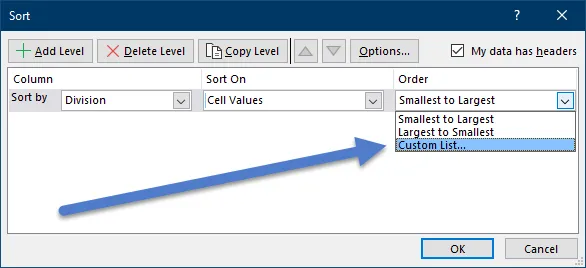
In the Custom List dialog box, enter the departments in the List Entries field in the order you prefer. Once the items have been entered, click the Add button to add them to the Custom Lists library.
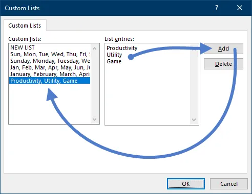
Click OK to apply the newly created custom list to your table.
Multiple-Level Sorting
When your list contains may duplicate entries for your primary sort column, it is common to sort each group of primary items by some secondary criteria. Example: we may wish to perform a primary sort by Company and then perform a secondary sort by Department. This way, each company’s departments are in alphabetical order.
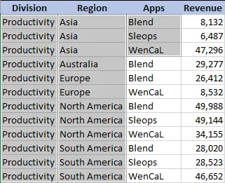
In our sample file, we want to perform a primary sort by the Division, and then perform a secondary sort by Region. We will take it a step further and perform a tertiary sort for each Region by their respective Apps.

We now see that all the Divisions are sorted alphabetically, and each Region is sorted alphabetically within their respective Division. Additionally, the Apps are sorted alphabetically within their respective Region.
Colors & Icons
Excel tables can also be sorted by the color of the cell, the color of the text, and the icon displayed in the cell via Conditional Formatting’s Icon Sets.
In the following image, the user has manually applied fill colors to various Revenue values. We would like to sort the list by the colored values first (red zone) and then sort the duplicate color rows by the original sort scheme of Division – Region – Apps (blue zone).
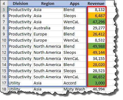
Because we have previously defined the “blue zone” logic, we will modify the existing sort scheme by right-clicking on the table and choosing Sort and then Custom Sort.
Insert two new sort levels by clicking the Add Level button two times. If the newly inserted levels do not appear at the top of the list, but rather mixed in with the original three sort options (see below), use the up and down arrows to reorder the criteria logic within the sort list.
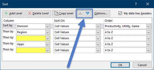
We will set the first sort criteria to examine the Revenue column. Instead of sorting on the cell’s value, we will sort on the cell’s color.
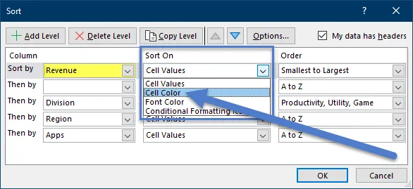
The sorting options will now change to allow us to select the color by which we want to sort.
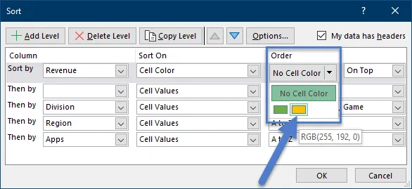
We can now repeat the process, selecting Revenue and Cell Color for the secondary sort but select a different color.
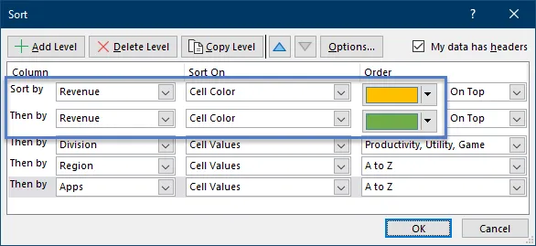
Once the sort routine has been applied, the result list appears as follows.
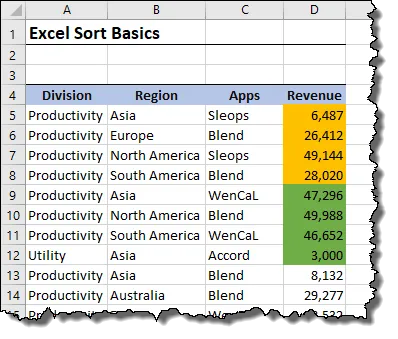
Sorting by Icons
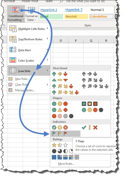
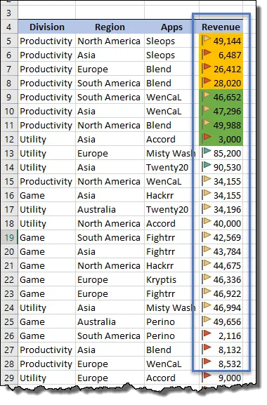
Using the results of the previous example, let’s use Conditional Formatting to add icons of colored flags to the values of the Revenue. Our logic will be that any value in the lower third of the set will display a red flag; any value in the upper third of the set will display a green flag; and all remaining middle‑third values will display a yellow flag.
Select all the Revenue values and choose Home – Conditional Formatting – Icon Sets – Flags.
Reopen the Custom Sort dialog box. We will remove the three sort levels that deal with Division, Region, and Apps. This is accomplished by selecting the desired level and clicking the Delete Level button.
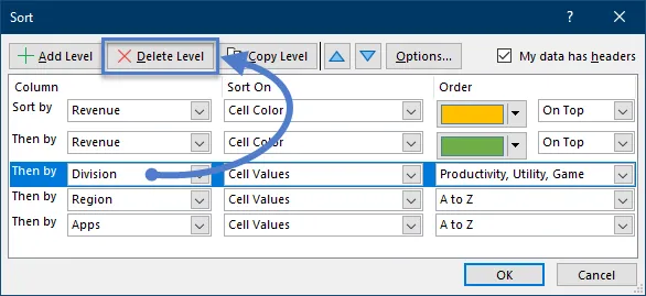
After deleting the three original sort levels, add three new sort levels and place them at the bottom of the sort list.
Set each of the three new levels to sort by Revenue. Set the Sort On options to sort by the green flag, then the yellow flag, and finally the red flag.
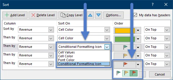
Observe that we are now sorting by cell color (all yellow then green) and then sorting by flag color (green then yellow then red.)
Unsort – Returning the List to Its Original Order
Suppose we wish to return the table back to its original order. The bad news is, in this example we can’t. Excel is not a database and does not retain any form of transaction record of where cells have moved. The moment you apply sorting to a list, the previous sort order is lost.
There is a technique you can implement if you wish to return to the original sort order.
IMPORTANT: This technique must be implemented PRIOR to any sorting that you wish to recover from.
The trick is to insert a column anywhere in your table (first, last, in the middle… it doesn’t matter) and create a list of sequential numbers. These numbers will act as an index to record the original row positions of the records prior to any sorting.
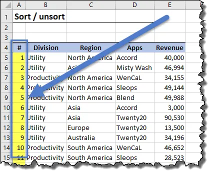
If you sort by any other column (i.e. descending by Revenue), the helper index column will become scrambled.
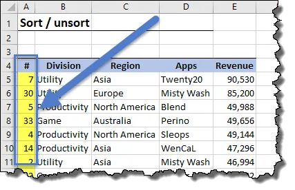
We can return to the original sort order at any time by resorting the list ascending by the helper index column.

Practice Workbook
Feel free to Download the Workbook HERE.

Leila Gharani
I'm a 6x Microsoft MVP with over 15 years of experience implementing and professionals on Management Information Systems of different sizes and nature.
My background is Masters in Economics, Economist, Consultant, Oracle HFM Accounting Systems Expert, SAP BW Project Manager. My passion is teaching, experimenting and sharing. I am also addicted to learning and enjoy taking online courses on a variety of topics.


