Suppose you have spent all day creating this amazing investment calculation tool that you plan to send to all members of your team.
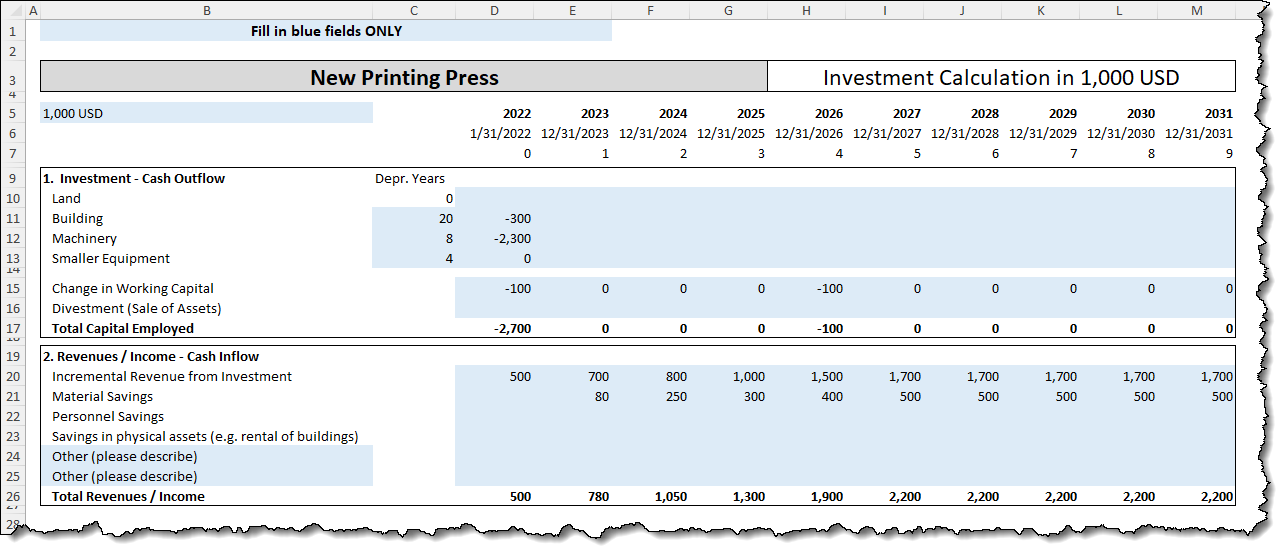
To direct users to the areas where they need to supply information to the calculator, we’ve shaded all input cells with a light blue fill and placed an instruction at the top telling the users to fill in the shaded blue cells only.
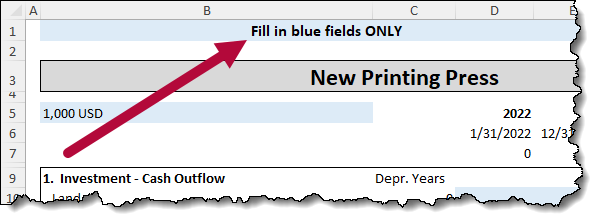
What is the probability that the users will attempt to click, type, or change non-blue shaded cells? My guess is 100%.
Let’s let the odds be ever in our favor (a little Hunger Games lingo).
Featured Course
Excel Essentials for the Real World

Protecting Cells From Unwanted Changes
To prevent a user from changing a cell’s content, like a cell holding a critical formula, we must execute a two-step process.
- Flag the cell as either a locked or unlocked
- Engage protection on the sheet.
When we perform the second step, protecting the sheet, any cell flagged as a locked cell will be protected from unwanted changes.
If we skip the first step, then all cells are flagged as locked by default. The entire sheet will be placed in a read-only mode when engaging sheet protection.
Attempting to change a protected cell’s contents will reveal the following message.

If we don’t want the entire sheet protected, we’ll need to “punch some holes” in our protective wall.
Step 1: Setting the Cell’s Protection Status
To set the status of a cell as either locked or unlocked we need to access the cell’s formatting controls.
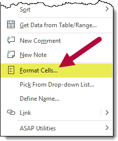
Highlight a cell or multiple cells, then right-click a selected cell and click Format Cells… . (You can also press CTRL-1 to open the needed dialog box.)
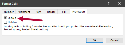
In the Format Cells dialog box, select the Protection tab. This will display the “Locked” property for the selected cell.
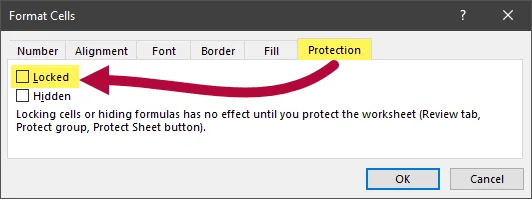
Placing a check will ensure the cell is locked when sheet protection is engaged.
Clearing the checkbox will ensure that the cell can be freely changed while protecting the remainder of the sheet’s cells.
NOTE: If you see a filled checkbox like below, it means that you have selected two or more cells that have a mixture of locked and unlocked states.
Many beginning users assume (and we know what happens when you assume) that just by checking the “Locked” box they have protected the cell from changes. This is incorrect.
You must perform the next step for protection to be enforced. All you have done here is tell Excel which cells to protect when performing the next step.
Step 2: Engaging Sheet Protection
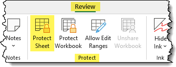
Once you have decided which cells will be protected and which cells will remain open to changes, engage sheet protection by selecting Review (tab) -> Protect (group) -> Protect Sheet.
A Protect Sheet dialog box appears asking for a password to unlock the sheet.
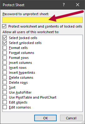
Protecting a sheet with a password is optional, but it’s a good way to keep a semi-literate Excel user from removing the sheet protection and making mischief with your file.
After you click OK, the sheet is now protected from unwanted changes in the entire spreadsheet while allowing changes to defined areas (i.e., exceptions).
Featured Course
Power Excel Bundle

Selecting Cells for Protecting Flagging
In our example, we have an unconventional range of cells that we need to select to exempt those cells from the protection rules.
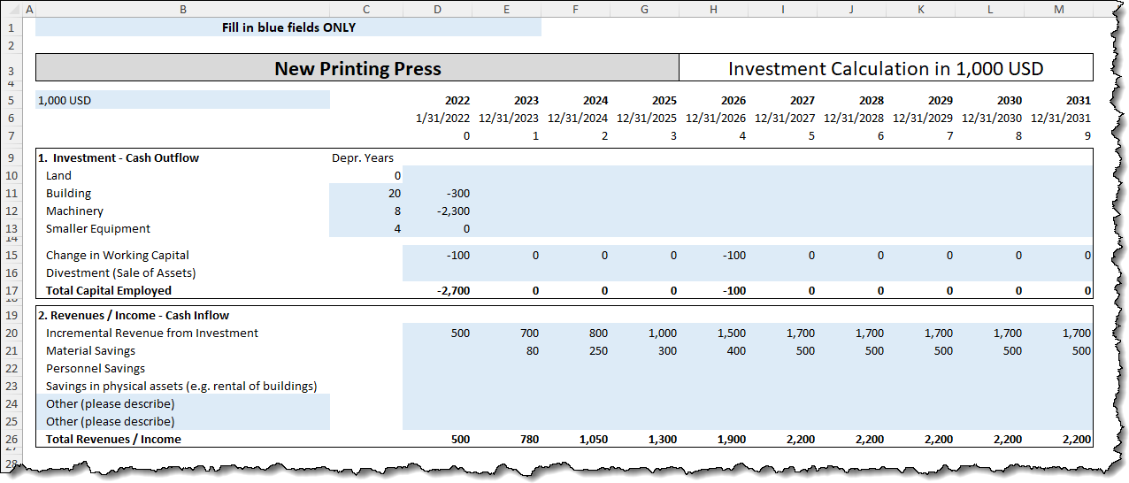
We could use some exotic click-CTRL-click strategy to select all the blue cells, but that would prove tedious and most likely frustrating.
Let’s have Excel select the blue cells for us.
Press CTRL-F to open the Find and Replace dialog box.
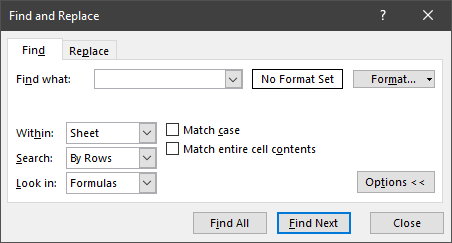
This tool is usually used to locate cells that contain specific text or to replace said text with different text.
We will use this tool to locate all cells with a blue fill color.
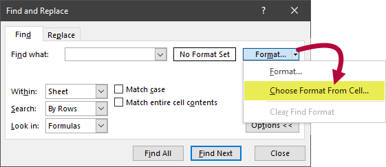
Click the small arrow to the right of the button that says Format… and select Choose Format From Cell… .
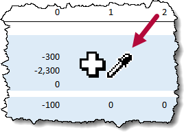
Your pointer will change to a fat plus with an eyedropper (pointer image below enlarged for clarity).
Click a cell that has the blue color then select Find All in the dialog box.
This will present a list with all cell locations matching the selected blue cell.
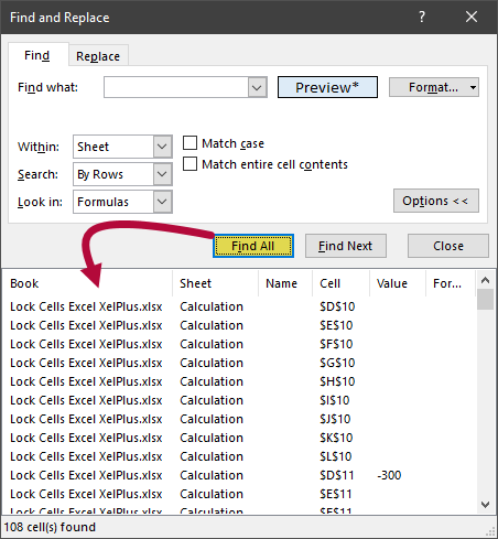
To select the discovered cells, click any cell reference in the list then press CTRL-A to select all cell references in the list.
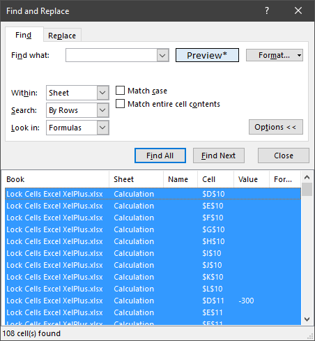
“What if I don’t find every blue cell in the list?”
If the Choose Format From Cell… fails to find every blue cell, it’s like due to some other setting that doesn’t match the cell’s properties. This option is not just looking for cells by color but rather by all matching cell properties.
If you want to locate cells only by their color and no other cell property, click the Format… button to open the Find Format dialog box and select the Fill tab.
From here, click the desired fill color and click OK.
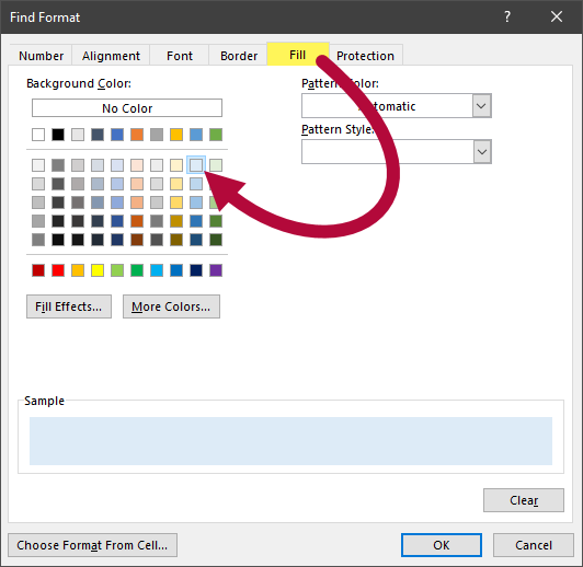
Now click Find All to repeat the same discovery and selection process from the earlier example.
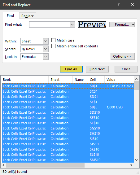
If unwanted cells have been inadvertently targeted by this process, you can hold the CTRL key and click the unwanted cells to deselect them from the targeting process.
NOTE: If you press CTRL-F later to perform a different selection routine, you are likely to have the previous setting still in effect. To clear any previous selection criteria, click the arrow to the right of the Format… button and select Clear Find Format.
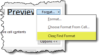
You are now properly positioned to press CTRL-1 to open the Format Cells dialog box and set the “Locked” property on the Protection tab accordingly.

Practice Workbook
Feel free to Download the Workbook HERE.

Leila Gharani
I'm a 6x Microsoft MVP with over 15 years of experience implementing and professionals on Management Information Systems of different sizes and nature.
My background is Masters in Economics, Economist, Consultant, Oracle HFM Accounting Systems Expert, SAP BW Project Manager. My passion is teaching, experimenting and sharing. I am also addicted to learning and enjoy taking online courses on a variety of topics.


