If you haven’t had a chance to read about Dependent Drop-down lists in Google Sheets, take a moment to click the image below to read (or watch) a complete discussion on this process.

Setting Up the Supporting Data
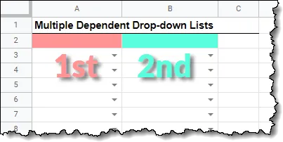
We have a spreadsheet where the first dropdown list will be created in cell A3 while the dependent (second) dropdown list will be created in cell B3.
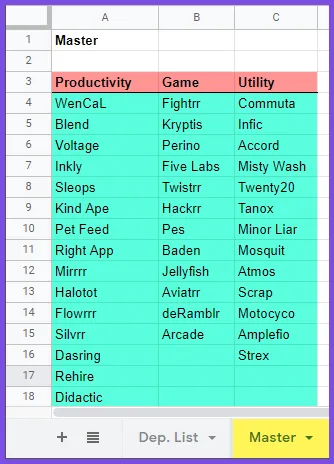
The lists for the two dropdowns are located on a sheet named “Master” where the first list points to the heading row of the table (cells A3:C3) and the second list points to the remaining items in the table (cells A4:C20). A few extra rows were selected to accommodate additions to the table.
Featured Course
Google Sheets – The Comprehensive Masterclass

Creating the First Dropdown List
To create the dropdown for Division, perform the following steps:
- Select cell A3.
- Select Data -> Data Validation.
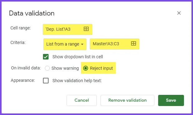
- In the Data Validation dialog box, select “List from a range” in the Criteria section and define the range as Master!A3:C3. We also wish to disallow any custom data from being entered into the cell, so we activate the “Reject input” option.
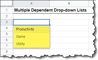
We can click the dropdown button located in cell A3 to reveal the following list of Divisions.
Google Sheets’ Interesting Behavior
If we were to copy cell A3, then paste the copied cell to range A4:A12, we see that the Data Validation logic is replicated across all pasted cells.
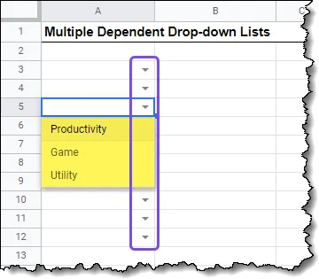
The interesting behavior is not so much about copying and pasting Data Validation. The interesting behavior is that the range reference for the list remained fixed even though we did not define it as an absolute reference in the criteria range.
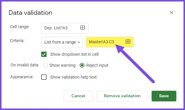
It seems like we would have been responsible for adding dollar signs in the reference to change it from a relative reference to an absolute reference.(i.e., A3:C3 to $A$3:$C$3).
Data Validation has automatically interpreted our range selection as an absolute reference, even though it was defined as a relative reference.
This is a welcomed courtesy for those not well versed in the difference between relative and absolute references, but it works against us later in our mission to create the additional dependent dropdown lists. Not to worry; we have a way around it.
Setting Up the Second (Dependent) Dropdown List
Now we create dropdown lists that are reactive to the first dropdown lists. These must work for each row independently of the adjacent rows.
Remember we only wish to display Apps that are associated with the selected Division from the first dropdown list.
Creating the Data Preparation Area
As Google Sheets will not allow us to create a formula directly in the cell where the dropdown is to exist, we will write the formula in a “helper column” and reference the results with Data Validation.
Creating an Index List
Returning to the “Master” sheet, we will create a list of numbers from 1 to 10 in cells E4:E13. Each of these numbers corresponds to a “first” dropdown on the input sheet.
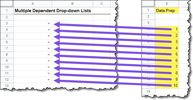
Creating the App Lookup List
To create a list of Apps that correspond to the user’s selection in the first dropdown (cell A3 – input sheet), select cell F4, and enter the following formula.
=INDEX($A$4:$C$20, , MATCH('Dep. List'!A3, $A$3:$C$3, 0) )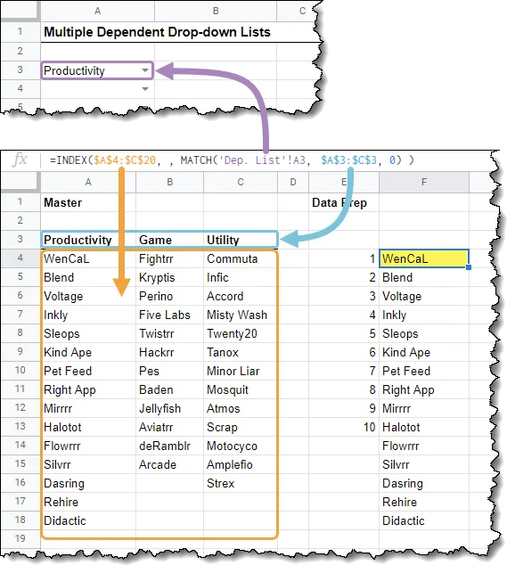
The result is a list of Apps from the selected Division.
To break the formula down into its pieces:
- The INDEX function uses the first argument to select the array of cells $A$4:$C$20.
- We want ALL ROWS to be returned, so we omit the second argument in the INDEX function, hence the 2 commas with nothing between them.
- The third argument uses a MATCH function to locate the item listed in cell A3 of the input sheet within the list of Department in cells $A$3:$C$3. This match must be an exact match, so a 0 is used to set this behavior in the MATCH
Transposing the Results
Because we want our results to be listed horizontally (across the row) instead of vertically (down the column), we will nest the entire INDEX/MATCH formula within a TRANSPOSE function.
=TRANSPOSE(INDEX($A$4:$C$20, , MATCH('Dep. List'!A3, $A$3:$C$3, 0) ) )
Filling Down for the Remaining Lists
If we take the formula created in cell F4 and fill it down to cell F13, we are presented with a panic moment.
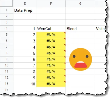
Not to worry. This is only because we have not selected any Divisions from the remaining dropdowns. These errors will disappear once we occupy the remaining division dropdowns.
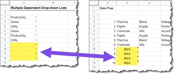
But who wants to look at errors that aren’t real errors?
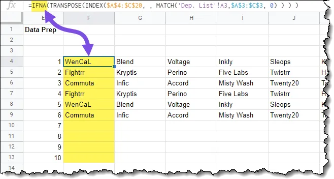
To suppress the #N/A error messages, we will nest the entire TRANSPOSE/INDEX/MATCH formula within an IFNA() function.
=IFNA(TRANSPOSE(INDEX($A$4:$C$20, , MATCH('Dep. List'!A3, $A$3:$C$3, 0) ) ) )If we replace the original TRANSPOSE formulas with the updated formula, we see the following results.
Enter the “Implied Absolute” Problem
We return to the input sheet to set up the dependent dropdown list for the Apps.
To create the dropdown for Division, perform the following steps:
- Select cell B3.
- Select Data -> Data Validation.
- In the Data Validation dialog box, select “List from a range” in the Criteria section and define the range as Master!F4:Z4. We also wish to disallow any custom data from being entered into the cell, so we activate the “Reject input” option. A few extra columns were selected to accommodate additions to the table.
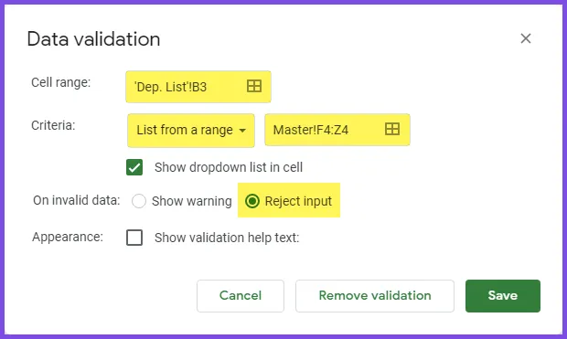
The result is a list of Apps for the selected Division.
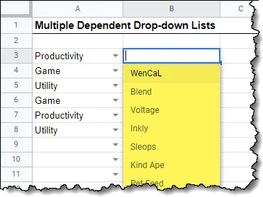
If we copy the B3 cell and paste it across the remaining Column B cells, we don’t get what we were expecting from the dependent dropdowns.
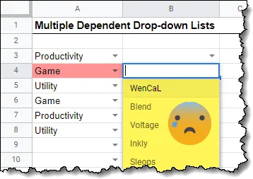
Every dependent dropdown has the list for whatever Division is selected in cell A3. This is because all dependent dropdown lists are looking at range F4:Z4 for their list of Apps.
This goes back to the implied absolute behavior mentioned earlier in the post. It worked to our advantage then, but now it presents us with a challenge to overcome.
This is a “good news/bad news” situation.
The good news is that the problem can be solved. The bad news is that it will require manual intervention to adjust to the Data Validation settings of each dependent dropdown list.
After having copied the Data Validation settings from cell B3 to cells B4:B12, select cell B4 and open the Data Validation dialog box.
In the Criteria section, change the row references to point to the next row. Instead of F4:Z4, the updated reference should read F5:Z5.

Continue to update the remaining rows, changing the Criteria option to examine the next row in the data preparation area (ex: F6:Z6, F7:Z7, F8:Z8 … F13:Z13).
Thoughts on this Process
If you only require a few rows (i.e., 10 or 20) of dependent dropdown lists, this wouldn’t take too long to construct. If you require hundreds or thousands of these, you may need to investigate writing an App Script to automate the creation process.
The benefit to having an App Script is that once it’s written, you can reuse it as many times as you need in new or existing projects.
Practice File
Feel free to get your own copy of the file HERE.

Leila Gharani
I'm a 6x Microsoft MVP with over 15 years of experience implementing and professionals on Management Information Systems of different sizes and nature.
My background is Masters in Economics, Economist, Consultant, Oracle HFM Accounting Systems Expert, SAP BW Project Manager. My passion is teaching, experimenting and sharing. I am also addicted to learning and enjoy taking online courses on a variety of topics.


