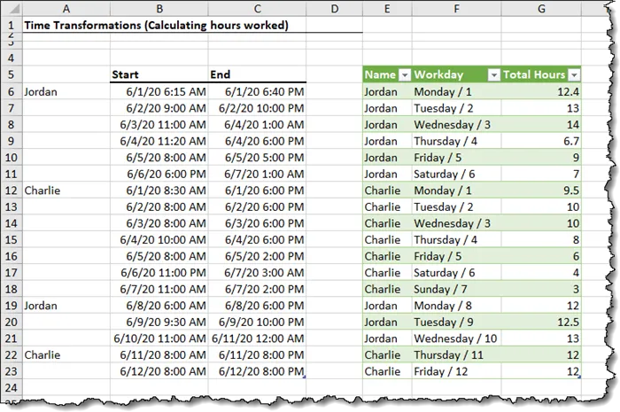
For our example, we have a list of users who record their hours worked by entering their start date/time and end date/time into separate columns. All successive rows of dates/times belong to the listed user until a new user’s name is encountered.
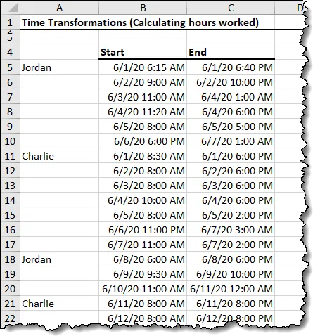
Our objectives are as follows:
- Calculate the number of hours worked for each entry.
- Which weekdays was the work performed?
- How much time was spent per person on the project?
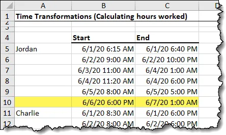
It is possible that a user could start working late one evening and work past midnight into the following day.
Preparing the Table
The first step is to “upgrade’ the plain table into a proper Excel Table.
Highlight cells A4 through C22 and press CTRL-T. We will not define a header row in the new table because we don’t want to change the format of the table.
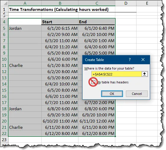
Press OK to complete the process.
We’ll also remove any of the newly applied colors by setting the table color to “None” from the Table Design (tab) -> Table Styles (group).

We want to use our original header and not the headers that came with the upgrade, so deselect “Header Row” from the Table Design (tab) -> Table Style Options (group).

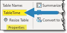
Lastly, we will give the table a proper name of “TableTime” in the Table Design (tab) -> Properties (group) -> Table Name field.
Featured Course
Master Excel Power Query – Beginner to Pro

Bring the Data into Power Query
Next, we’ll bring the upgraded table into Power Query by selecting Data (tab) -> Get & Transform Data (group) -> From Table/Range.

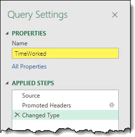
Name the new query “TimeWorked” in the Query Settings -> Properties -> Name field.
Initial “Fixes”
The data types seem to have been detected correctly as Date/Time and the column of names as Text.

We will give the first column a better name of “Name”.

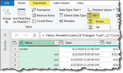
We will repeat the names for each successive empty row with the name that appears above the empty cells. We can do this by selecting Transform (tab) -> Any Column (group) -> Fill -> Down.
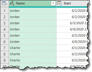
The column now appears as such where each row of times is associated with a user’s name.
Performing Time Transformations
You can find the Time transformation tools on both the Transform tab and the Add Column tab.

Be careful which you use. Even though the options are labeled the same, the result will be markedly different.
The general rule of thumb is: If you use a feature from the Transform tab, you are REPLACING old data with altered data. If you us a feature from the Add Column tab, you are preserving the old data and creating additional columns of information.
Extracting the Time
Below are a few examples of how you can manipulate the Time from a Date/Time field.
If we want to extract the time component of the “Start” column’s Date/Time, select the “Start” column and click Add Column (tab) -> Date & Time Column (group) -> Time -> Time Only.

Extract the Beginning of the Hour
For those entries where the user did not start their work at the exact start of the hour, we can “round down” to the nearest hour by selecting Add Column (tab) -> Date & Time Column (group) -> Time -> Hour -> Start of Hour.

We get the same Date/Time information, but the times have been reduced to the closest hour.
Extracting the Minutes or Seconds
If you need to extract a single component of the time, like the Hour, the Minute, or the Second, you can select Add Column (tab) -> Date & Time Column (group) -> Time -> Hour / Minute / Second.

Solving for Time Worked
To answer our first question, “How much time did each user work per session?”, we will perform the following actions.
- Select the “End” column
- Press the CTRL (or Shift)
- Select the “Start” column
NOTES: We are selecting the “End” column first because we want our logic to read “End minus Start”. If we select the columns in the reverse order, we will end up with negative times.
- Select Add Column (tab) -> From Date & Time (group) -> Time -> Subtract.
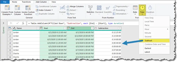
NOTE: If the option for “Subtract” is not available (grayed-out), it is likely because the two columns of times were not selected. Return to Step 1 and try again.
The result is set as a Duration data type.

The Duration data type is represented as the length of time shown as days, hours, minutes, and seconds.
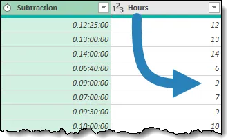
Days.Hours:Minutes:SecondsTo display the result as a number of hours worked, select the results column and click Add Column (tab) -> From Date & Time (group) -> Duration -> Hours. The results are hours rounded down to the nearest hour.
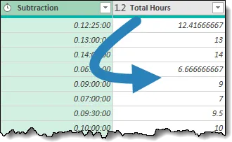
If we were to select Add Column (tab) -> From Date & Time (group) -> Duration -> Total Hours, the result will be the precise number of hours (to the second.)
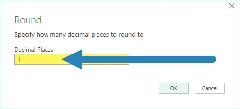
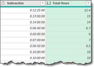
By using the Total Hours option, we can then round to the nearest hour in both directions by selecting the Total Hours column and clicking Transform (tab) -> Number Column (group) -> Rounding -> Round and select 1 as the decimal place value.
This gives us the results we need.
Discovering the Weekdays Worked
Our next objective is to determine which weekdays the users worked.
This is accomplished by extracting the weekday name from the “Start” column.
Select the “Start” column and click Add Column (tab) -> From Date & Time (group) -> Date -> Day -> Name of Day.

To make the results easier to read, we would like to have the day number next to the name of the day (ex: Wednesday / 3).
Select the “Start” column and click Add Column (tab) -> From Date & Time (group) -> Date -> Day -> Day.

Now we will merge these column results by performing the following steps.
- Select the Day Name and the Day columns (using CTRL or Shift) and click Transform (tab) -> Text Column (group) -> Merge Columns.
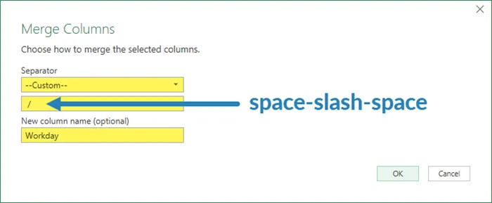
- In the Merge Columns dialog box set the Separator to “Custom” and set the separator to “ / “ (this is a space-forward slash-space combination).
- Name the new column “Workday” and press OK.
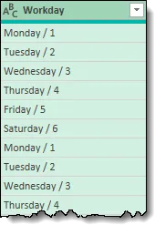
The result is a much easier to read set of dates.
Featured Course
Power Excel Bundle

Remove the Unnecessary Fields
We will only keep the results of our above work, so select the “Start”, “End”, and Subtraction” fields from the table and press the Delete key on the keyboard.
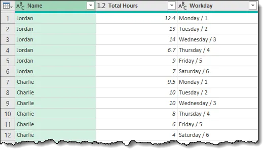
Relocate the “Work Day” field to rest between the “Name” and “Total Hours” columns. Click and hold the heading for the “Work Day” field and drag the field to fall between the first two fields.
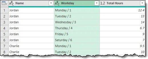
With our table finished, we will load the results into an Excel Table next to the original data.
- Select Home (tab) -> Close (group) -> Close & Load -> Close & Load to…
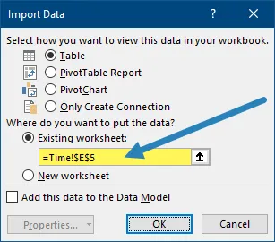
- In the Import Data dialog box, select Table and Existing Worksheet to point to cell E5.
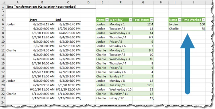
We see the original data next to the modified data.
Calculate Total Time per User with Group By
Our final objective is to calculate the total number of hours worked for each user.
We want to group the results table by “Name” and aggregate (SUM) the “Total Hours”.
We aren’t interested in the “Work Days” column, so we will remove it from the new result.
Instead of creating a new query and repeating most (if not all) of the first query’s steps, we will create a second query that references the first query. Think of it as “the first query’s output will be the second query’s input”.
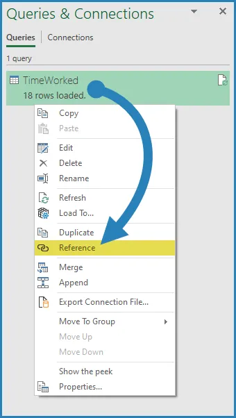
- In the Queries & Connections panel, right-click the “TimeWorked” query and select Reference.
- Rename the new query “TotalTime”.
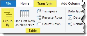
- With the “Name” field selected, click Transform (tab) -> Table (group) -> Group By.
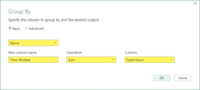
- In the Group By dialog box, set the field to be grouped as “Name”, the new column name to “Time Worked”, and set the operation to Sum using the “Total Hours” field.
- Click OK to view the results.

- As a bonus step, we will round the “Time Worked” results up to the nearest hour by selecting the “Time Worked” field and clicking Transform (tab) -> Number Column (group) -> Rounding -> Round Up.

With our grouped table finished, we will load the results into an Excel Table next to the results of the first query.
- Select Home (tab) -> Close (group) -> Close & Load -> Close & Load to…
- In the Import Data dialog box, select Table and Existing Worksheet to point to cell I5.
Updating with New User Times
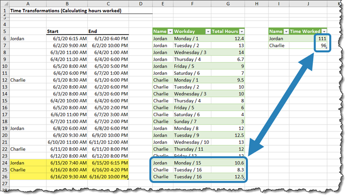
If the users continue to add days worked, we want to ensure that our query results will see the newly added information.
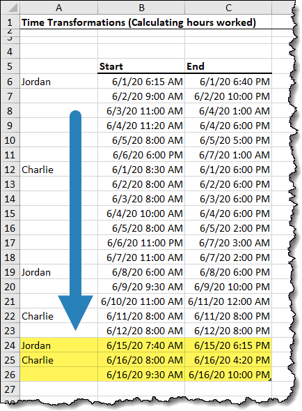
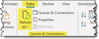
To refresh the query output, select either of the results tables and click Data (tab) -> Queries & Connection (group) -> Refresh All.
We see the newly added times in our reports.
Practice Workbook
Feel free to Download the Workbook HERE.

Leila Gharani
I'm a 6x Microsoft MVP with over 15 years of experience implementing and professionals on Management Information Systems of different sizes and nature.
My background is Masters in Economics, Economist, Consultant, Oracle HFM Accounting Systems Expert, SAP BW Project Manager. My passion is teaching, experimenting and sharing. I am also addicted to learning and enjoy taking online courses on a variety of topics.


