Method #1: Flash Fill
Flash Fill (introduced in Office 2013) is one of Excel’s greatest tools for modifying data based on a pattern.
Suppose we have a list of numbers, and we need to append the text “ID” to the beginning of each number.
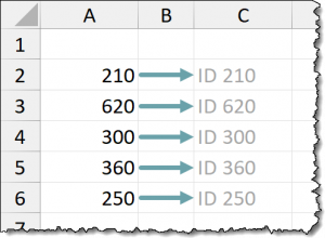
With Flash Fill, you just need to provide Excel with an example of what you wish you had. In this case, on the same row and directly next to the original data, “I wish I had ‘ID 250’ “.
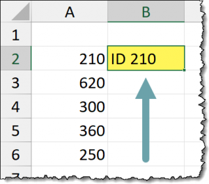
Next to the second item in the list, begin typing what would be the next thing “you wish you had”.
Not too far into the example, a ghostly list of suggestions will appear.
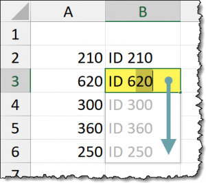
If you are happy with the offerings, press ENTER to commit the remainder of the list.
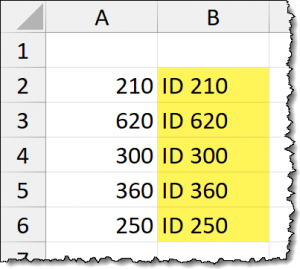
Granted, this is a very short list, and you could have likely type it just as fast, but you must keep in mind that this would have worked the same way for 500,000 items in the list as easily as it worked for 5.
Alternate Flash Fill Method
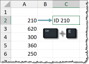
Another way of invoking Flash Fill is to press CTRL-E after you have entered the first example.
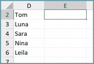
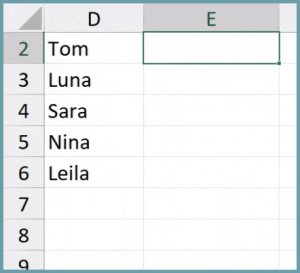
We can do the same thing with text. If we have a set of names, and we want to place the characters “ID-“ before each name, type an example of “what you want” next to the first entry in the list and press CTRL-E.
Featured Course
Excel Essentials for the Real World

Method #2: Using Formulas
One of the weaknesses of Flash Fill is that the results aren’t dynamic. Once they are produced, the results don’t change if the source data changes.
If you are using data that changes and those changes need to be reflected in the revised version, you will need to utilize formulas.
To formulaically (fancy word alert) append the text “ID” to the beginning of the values, we would write a formula like the following.
="ID " & A2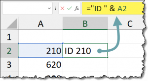
Pay special attention to the included space character after the letters “ID”. This is to include a small amount of visual padding between the letters “ID” and the numbers that follow.
Use Fill Series to replicate the formula to the adjacent rows and we have our modified data.
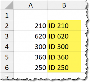
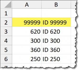
The advantage of this method is that if one of the source values (Column A) changes, we get an immediate update in the formula results (Column B).
Adding Text to the END of Values
If you need to append text to the end of the data, you can continue the same operation but with the text at the end of the formula instead of the beginning.
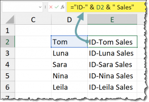
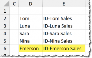
BONUS: If you used Flash Fill to produce the “before and after text” example, and the data changed, you can manually update the result by doing the following:
- Highlight and delete the original results.
- Click next to the first item in the list and type “ID Tom Sales” and press ENTER.
- Press CTRL-E to invoke the Flash Fill
Featured Course
Master NEW Excel Functions in Office 365 & Office 2021

Method #3: Custom Number Formatting
The Custom Number Formatting feature in Excel is all about making data appear in a specific way.
Most users are familiar with formatting presets like the “Long Date” style, the “Currency”, style, and the “Text” style just to name a few.
But what many users are not aware of is that you can supplement existing data with additional text and numbers.
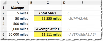
Imagine a spreadsheet where the users enter a mileage value and the text “miles” is displayed next to the number in the same cell.
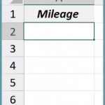
Using our previous example’s data, we can select the data and press CTRL-1 to open the Number Formatting dialog box.
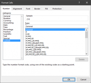
Selecting the category CUSTOM, we can define the formatting of our choosing.
If we want to place the letters “ID “ (with a space at the end) we would enter the text in double-quotes and follow the text with a “#” character (no quotes).
"ID "#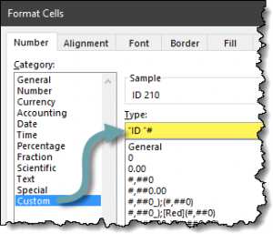
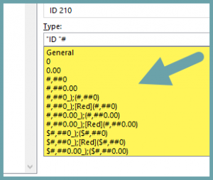
If you want to implement thousands separators or decimal points for fractions, you can use of codesets listed in the same window.
Clicking OK reveals the newly formatted data.
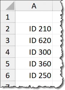
The great advantage to Custom Number Formatting is that the numbers remain numbers and can be utilized in calculations. Looking back at the mileage example, it is still possible to calculate the total and average miles of the set.
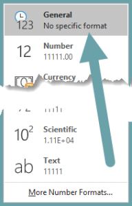
If you need to remove the custom formatting from the data, you can set the cell’s style to GENERAL.
“But what about formatting a text entry?”
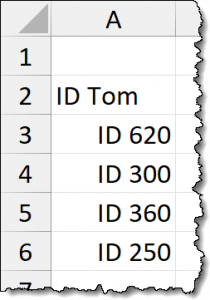
We can see that by placing the text “Tom” in a previously formatted cell, the custom formatting does not carry over.
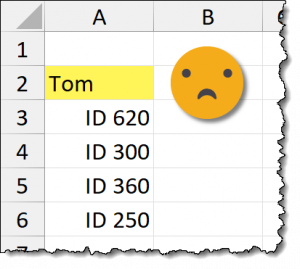
This is because we defined a custom formatting rule for the numbers (more specifically, the positive numbers) but not for the text.
We can update the Custom Number Formatting to have a rule for the numbers as well as the text.
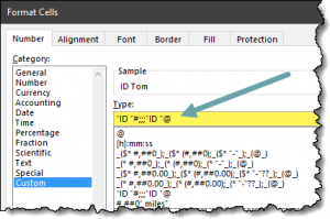
"ID "#;;;"ID "The three semicolons are there to act as placeholders as we are not defining formatting for negative values or zeroes.
NOTE: For a detailed explanation of the Custom Number Formatting codes along with practical examples, check out the link below.
Learning Excel Custom Number Formatting
Why you SHOULD be USING Custom Number Formatting
The Choice is Yours
Each of these techniques has its inherent advantages and disadvantages.
The main factors that will factor into your choice are:
- Do you need the results to be dynamic?
- Do you need to perform a calculation on the formatted data?
- Are you comfortable with custom number codes?
Practice Workbook
Feel free to Download the Workbook HERE.

Leila Gharani
I'm a 6x Microsoft MVP with over 15 years of experience implementing and professionals on Management Information Systems of different sizes and nature.
My background is Masters in Economics, Economist, Consultant, Oracle HFM Accounting Systems Expert, SAP BW Project Manager. My passion is teaching, experimenting and sharing. I am also addicted to learning and enjoy taking online courses on a variety of topics.


